A scalable diagonalization framework for tensor-product bitstring selected configuration interaction

I have a new paper to share that has been published in the Journal of Chemical Physics entitled a scalable diagonalization framework for tensor-product bitstring selected configuration interaction. This is the first paper I have ever been part of that is about the Selected Configuration Interaction (SCI) technique. It was very interesting to learn about it, and work with first author Dr. Enhua Xu on pushing the method on supercomputer Fugaku.

In quantum chemistry simulations, we often talk about two kinds of correlation: static and dynamic (or strong and weak correlation). SCI is a powerful method for static correlation, as it describes the multiconfigurational nature of the wavefunction. Meanwhile, dynamic correlation is typically treated well by many-body perturbation theory (such as coupled-cluster).

A classic example of static correlation is the breaking of N2's triple bond.

from pyscf import cc, gto, mcscf, mrpt, scf
distances = [0.80, 0.85, 0.90, 0.95, 1.00, 1.05, 1.10, 1.15, 
    1.20, 1.30, 1.40, 1.50, 1.60, 1.70, 1.80, 1.90, 2.00, 
    2.15, 2.30, 2.45, 2.60, 2.80, 3.00, 3.25, 3.50, 3.75, 4.00]

When we want to compute something accurately, our first instinct is to reach for coupled-cluster theory (the "gold standard" in quantum chemistry).

mf_list, rhf_e, ccsd_e, ccsdt_e = [], [], [], []
t1 = t2 = None

for r in distances:
    mol = gto.M(atom=f"N 0 0 0; N 0 0 {r}",
                basis="cc-pVDZ", unit="Angstrom",
                symmetry="D2h", verbose=0)
    mf = scf.RHF(mol).run()
    mycc = cc.CCSD(mf, frozen=2)
    mycc.kernel(t1=t1, t2=t2)
    et = mycc.ccsd_t()
    mf_list.append(mf)
    rhf_e.append(mf.e_tot)
    ccsd_e.append(mycc.e_tot)
    ccsdt_e.append(mycc.e_tot + et)
    t1, t2 = mycc.t1, mycc.t2

Here we reuse our t1/t2 amplitudes as an initial guess because some of the stretched geometries are difficult to converge. Plotting the result:

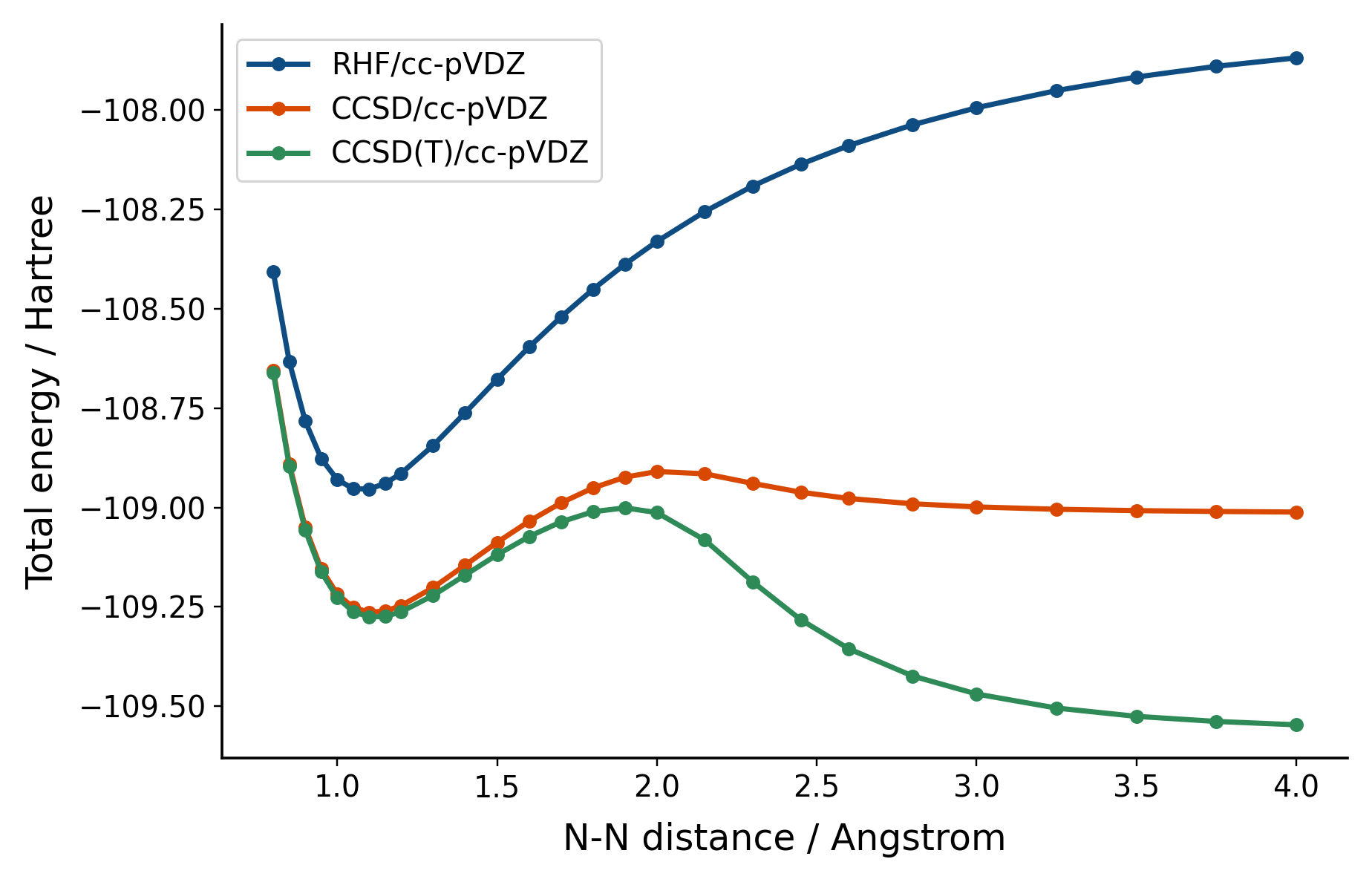
What we see here is coupled-cluster theory failing dramatically. Not only is CCSD showing weird behavior as we stretch the bond, but CCSD(T) - which should be better right? - gets even worse. This is because we have a system with a lot of static correlation, but are using a theory that is mainly capturing dynamic correlation.

The solution is to describe this system as multi-reference. One tool we can use is CASSCF, here using a small active space for practical purposes:

mc_list, casscf_e = [], []

for mf in mf_list:
    mc = mcscf.CASSCF(mf, 6, 6)
    mc.kernel()
    mc_list.append(mc)
    casscf_e.append(mc.e_tot)

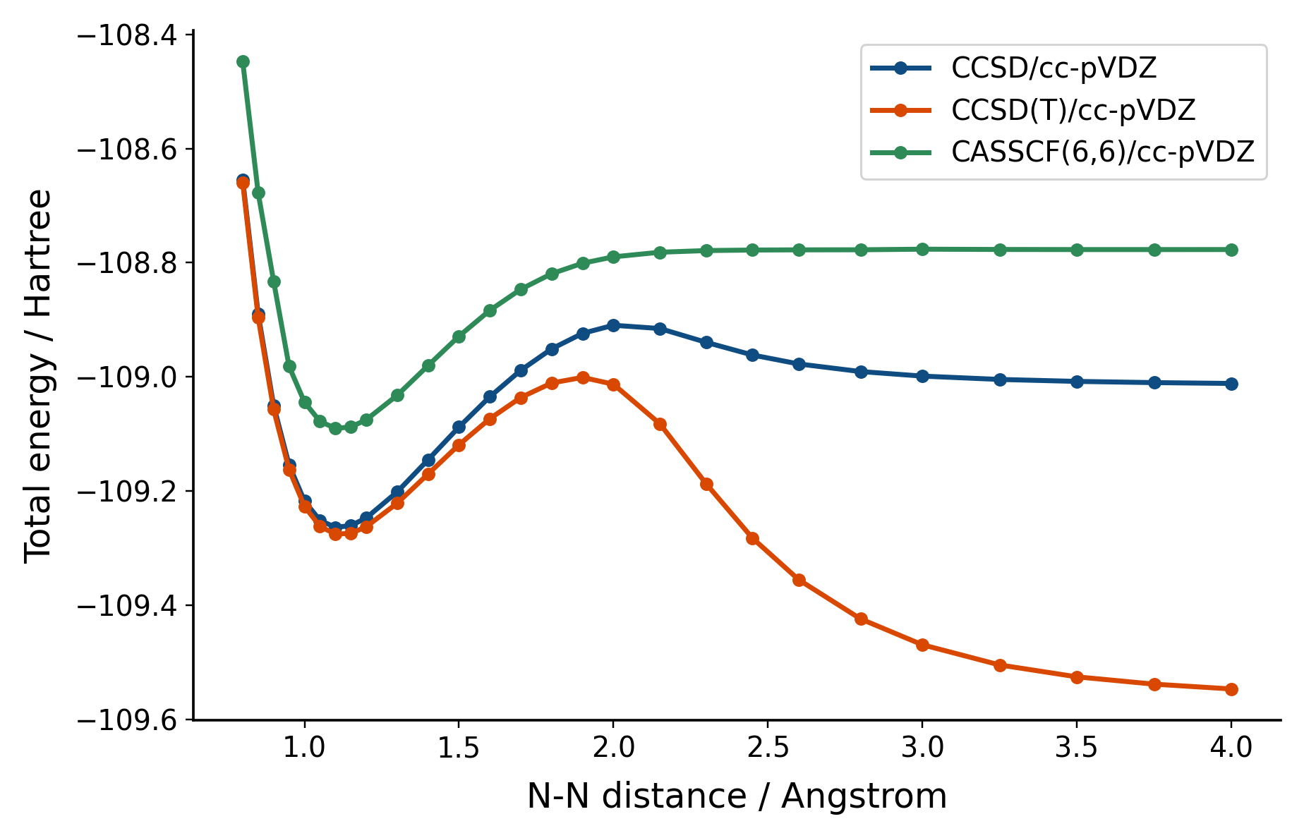Adding CASSCF to the mix, we find that much more reasonable behavior at the disassociation limit. Yet the depth of its well at equilibrium is not as deep as CCSD. While coupled cluster is not variational, we can't help but be suspicious. Indeed, is because with CASSCF we can describe the static correlation well, but is missing the dynamic correlation.

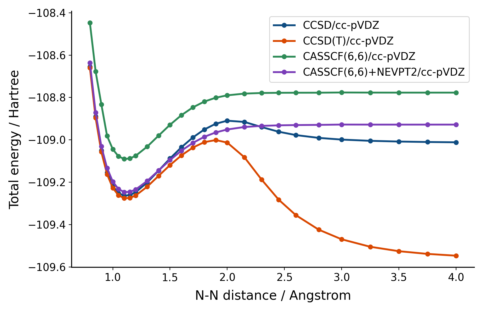
To improve on the result, we could of course increase the active space size towards Full Configuration Interaction. But another way is to combine perturbation theory with configuration interaction using NEVPT2.

nevpt2_e = [mc.e_tot + mrpt.NEVPT(mc).kernel() for mc in mc_list]

If these kinds of challenging problems interest you, and you want to go far beyond the scale your laptop allows, I hope you check out our paper!