A Simple Solver In Python
In this blog post, I would to introduce a simple Schrödinger equation solver in python. There are of course plenty of programs out there that can solve the Schrödinger equation. And many of them solve it in the context of practical theories and systems. However, often times the resulting wavefunctions of those calculations are deeply hidden within the program, which makes it tedious to experiment with. When I'm trying to do something new, sometimes I'll turn to this kind of simple program.
I'm going to write here what I think is the absolute bare minimum solver you can make. We'll only solve equations in one dimension. We'll use the eigensolver provided by SciPy. And we'll solve all the equations in real space using the finite difference method. First, let's recall the time independent Schrödinger equation:
$$\begin{equation} \big[\nabla^2 + V(x)\big] \psi = \lambda \psi. \end{equation}$$
First let's process the input. Ignore some of the import statements for now, we'll come back to these functions when we use them.
from sys import argv
from numpy import linspace, diag
from scipy.sparse.linalg import eigsh
from matplotlib import pyplot as plt

from UniversalOperators import TOperator
import SystemOperators

if __name__ == "__main__":
    # Process Input
    grid_size = int(argv[1])
    nocc = int(argv[2])
    PotentialName = argv[3]
    x_values = linspace(-6.28, 6.28, grid_size)
    grid_spacing = x_values[1] - x_values[0]
Our program takes three input parameters:
- The number of grid points.
- The number of eigenvectors to compute.
- The name of the potential we want to study.
Using the linspace function in numpy, we can easily generate a list of evenly spaced grid points to represent our potential and wavefunction on.
Next we need a matrix that represents the kinetic energy:
    # Build Operator
    KineticMatrix = TOperator(grid_size, grid_spacing)
The Kinetic Energy operator is a universal operator, as opposed to the potential energy operators which are specific to the system we are trying to model. We will put the kinetic energy operator in a file UniversalOperators.py and the potential energy operators in SystemOperators.py. The kinetic energy operator can be implemented using the five point stencil approximation[1]:
from scipy.sparse import coo_matrix

def TOperator(grid_size, grid_spacing):
    '''
    Five point stencil kinetic energy operator.
    '''
    data = []
    row = []
    col = []

    for i in range(grid_size):
        if i > 1:
            row.append(i)
            col.append(i - 2)
            data.append((-0.5) * (-1.0 / (12.0 * grid_spacing**2)))
        if i > 0:
            row.append(i)
            col.append(i - 1)
            data.append((-0.5) * (16.0 / (12.0 * grid_spacing**2)))
        row.append(i)
        col.append(i)
        data.append((-0.5) * (-30.0 / (12.0 * grid_spacing**2)))
        if i + 1 < grid_size:
            row.append(i)
            col.append(i + 1)
            data.append((-0.5) * (16.0 / (12.0 * grid_spacing**2)))
        if i + 2 < grid_size:
            row.append(i)
            col.append(i + 2)
            data.append((-0.5) * (-1.0 / (12.0 * grid_spacing**2)))

    return coo_matrix((data, (row, col)), shape=(grid_size, grid_size))
In this routine, all the logic like if i > 0 is to deal with the boundary condition. In this simple example, the boundary condition is that the wavefunction goes to zero. Next we'll also have to construct a potential energy operator, and add it to our overall Hamiltonian:
    try:
        PotentialOperator = getattr(SystemOperators, PotentialName)
    except:
        exit(1)
    PotentialMatrix, potential = PotentialOperator(x_values)
    Hamiltonian = KineticMatrix + PotentialMatrix
Here we'll take advantage of Python's flexibility. The getattr function will get the function in the SystemOperators.py based on the string provided to the program. How should we implement these potential energy operators? Here's are two examples:
'''
Generate operators representing various systems.
'''
from scipy.sparse import coo_matrix
from scipy import exp
from scipy.special import lambertw

def HydrogenOperator(x_values):
    '''
    Hydrogen potential well
    '''
    grid_size = len(x_values)
    data = []
    row = []
    col = []

    for i in range(0, grid_size):
        row.append(i)
        col.append(i)
        x = x_values[i]
        data.append(1.0/abs(x))

    return coo_matrix((data, (row, col)), shape=(grid_size, grid_size)), data

def LambertOperator(x_values):
    '''
    Lambert W Function
    '''
    grid_size = len(x_values)
    data = []
    row = []
    col = []

    for i in range(0, grid_size):
        row.append(i)
        col.append(i)
        x = x_values[i]
        data_point = (1.0/(1.0 + lambertw(exp(-abs(x))))).real
        data.append(data_point)

    return coo_matrix((data, (row, col)), shape=(grid_size, grid_size)), data
The HydrogenOperator function is just a simple $\frac{1}{r}$ operator. The LambertOperator uses the Lambert W function[2] just to keep things interesting.
Now that we have the operator in matrix form, we can solve for the eigenvectors.
    # Solve The Eigenvalue Equation
    values, vectors = eigsh(Hamiltonian, k=nocc, which='SA')
And we can plot the result.
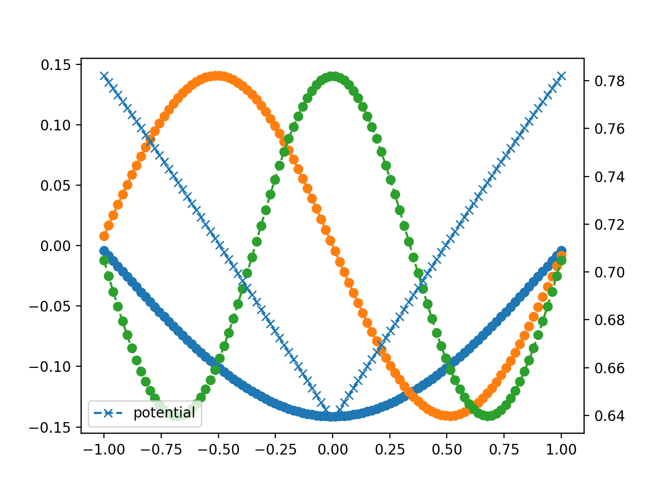
    # Plotting
    fig, ax1 = plt.subplots()
    ax2 = ax1.twinx()
    for i in range(0, nocc):
        ax1.plot(x_values, vectors.T[i], 'o--', label="K="+str(i))
    ax2.plot(x_values, PotentialMatrix.diagonal(), 'x--', label="potential")

    plt.legend()
    plt.show()
Some example output is below. We'll come back to this example later for some more interesting exercises.
[1] https://en.wikipedia.org/wiki/Five-point_stencil
[2] https://en.wikipedia.org/wiki/Lambert_W_function