Complexity Reduction in Density Functional Theory: Locality in Space and Energy
I am happy to announce a new paper in our series on Complexity Reduction. The title is "Complexity Reduction in Density Functional Theory: Locality in Space and Energy". In this sequence of papers, we've been trying to look at how to perform DFT calculations on large systems, with a focus on how to analyze large systems. In this paper, I incorporated our framework into a code called NTChem, which is based on Gaussian orbitals. NTChem has two major benefits over the previous code we integrated it with (BigDFT): hybrid functionals and an all-electron representation. This gave us some new things to explore.
For example: eigenvalues. I write in my papers a lot about how challenging it is to compute the eigenvectors/eigenvalues of large matrices right? Well, let's take a look at something really quick in PySCF.
from pyscf import gto
from pyscf import scf
mol = gto.M(atom = 'O         -1.17120        0.29970        0.00000; '
                   'H         -1.12910        0.83640        0.80990; '
                   'C         -0.04630       -0.56650        0.00000; '
                   'H         -0.09580       -1.21200        0.88190; '
                   'H         -0.09520       -1.19380       -0.89460; '
                   'H          2.10500       -0.37200       -0.01770; '
                   'H          1.24260        0.93070       -0.87040; '
                   'H          1.26160        0.90520        0.88860; '
                   'C          1.21750        0.26680        0.00000; ',
            verbose=0, basis = 'STO-3G')
mf = scf.RHF(mol)
_ = mf.kernel()
We will need the Hamiltonian and overlap matrices.
S = mf.get_ovlp()
H = 27.2114 * mf.get_fock() # Convert to eV
We can manually get the eigenvalues of these matrices by calling scipy's eigh.
from scipy.linalg import eigh
w, _ = eigh(H, b=S)
Now for the fun part. I'm going to print out the Hamiltonian matrix. Look at it closely. Can you guess what is the smallest eigenvalue of this matrix?
for row in H:
    print(" ".join(["%.0f" % x for x in row]))
-551 -140 -1 0 -1 -31 -0 -14 18 -14 -0 -3 -3 -0 -1 -0 0 -1 2 -0 -0
-140 -67 -2 0 -2 -27 -6 -17 16 -12 -0 -4 -4 -0 -1 -1 -0 -2 3 0 -0
-1 -2 -10 -1 0 -2 -9 -11 5 -8 -0 -3 -3 -0 -1 -1 -0 -2 3 0 -0
0 0 -1 -10 1 -7 7 8 -7 1 0 3 3 0 -0 -0 0 0 -1 -1 -0
-1 -2 0 1 -10 -12 -0 -1 1 -1 -5 -1 1 -0 0 -0 -0 -0 0 0 -1
-31 -27 -2 -7 -12 -15 -3 -7 5 -5 -2 -3 -2 -0 -1 -2 -1 -2 2 -0 -1
-0 -6 -9 7 -0 -3 -302 -81 0 -0 -0 -21 -21 -2 -2 -2 -0 -10 13 9 -0
-14 -17 -11 8 -1 -7 -81 -44 0 -1 -0 -20 -20 -5 -5 -5 -9 -16 13 8 -0
18 16 5 -7 1 5 0 0 -10 -0 0 1 1 -5 -4 -4 -13 -12 5 6 -0
-14 -12 -8 1 -1 -5 -0 -1 -0 -10 -0 7 7 -1 -4 -4 -9 -8 6 -0 -0
-0 -0 -0 0 -5 -2 -0 -0 0 -0 -9 -10 10 0 2 -2 -0 -0 0 0 -4
-3 -4 -3 3 -1 -3 -21 -20 1 7 -10 -13 -7 -2 -1 -2 -2 -5 4 3 -2
-3 -4 -3 3 1 -2 -21 -20 1 7 10 -7 -13 -2 -2 -1 -2 -5 4 3 2
-0 -0 -0 0 -0 -0 -2 -5 -5 -1 0 -2 -2 -13 -7 -7 -21 -20 -10 7 0
-1 -1 -1 -0 0 -1 -2 -5 -4 -4 2 -1 -2 -7 -13 -7 -20 -20 -0 -7 10
-0 -1 -1 -0 -0 -2 -2 -5 -4 -4 -2 -2 -1 -7 -7 -13 -20 -20 -0 -7 -10
0 -0 -0 0 -0 -1 -0 -9 -13 -9 -0 -2 -2 -21 -20 -20 -300 -81 -0 -0 -0
-1 -2 -2 0 -0 -2 -10 -16 -12 -8 -0 -5 -5 -20 -20 -20 -81 -43 1 0 -0
2 3 3 -1 0 2 13 13 5 6 0 4 4 -10 -0 -0 -0 1 -9 -0 0
-0 0 0 -1 0 -0 9 8 6 -0 0 3 3 7 -7 -7 -0 0 -0 -8 0
-0 -0 -0 -0 -1 -1 -0 -0 -0 -0 -4 -2 2 0 10 -10 -0 -0 0 0 -8
Hopefully you didn't start writing some code, or reach for a pen and paper, because the answer is simple.
from numpy import diag
from matplotlib import pyplot as plt
fig, axs = plt.subplots(1, 1, figsize=(4, 3))
axs.plot(w, 'x', label="Generalized")
axs.plot(sorted(diag(H)), '+', label="Diagonal of H")
axs.set_ylabel("Energy (a.u.)", fontsize=14)
axs.set_xlabel("IDX", fontsize=14)
_ = axs.legend()
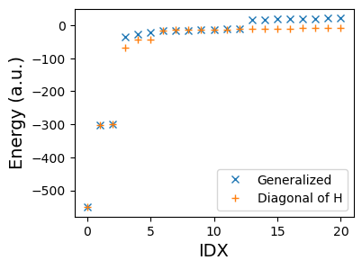
It's just the smallest element on the diagonal. That wasn't so hard was it?
...
Ok, of course, that's not exactly right.
print("Error:", sorted(diag(H))[0] - w[0], 'eV')
Error: 0.23812229157852016 eV
Can we do better? Using the STO-3G basis set, there are 5 basis functions associated with the Oxygen atom. Let's extract the submatrices associated with those basis functions.
idx = range(0, 5)
subH = H[idx, :][:, idx]
subS = S[idx, :][:, idx]
Next diagonalize those matrices. 3x3 is perfect for pen and paper.
ws, _ = eigh(subH, b=subS)
fig, axs = plt.subplots(1, 1, figsize=(4, 3))
axs.plot(w, 'x', label="Generalized")
axs.plot(sorted(diag(H)), '+', label="Diagonal of H")
axs.plot(ws, '.', label="Eigenvalues of subH")
axs.set_ylabel("Energy (a.u.)", fontsize=14)
axs.set_xlabel("IDX", fontsize=14)
_ = axs.legend()

print("Error:", ws[0] - w[0], 'eV')
Error: 0.026186869587604633 eV
That's a significant improvement, and we can do even better. The oxygen in Ethanol is bonded to a hydrogen atom (1 basis function) and a carbon atom (5 basis functions), which I carefully put in that order in the atomic structure. What happens if we add the hydrogen to our submatrix?
idx = range(0, 6)
subH2 = H[idx, :][:, idx]
subS2 = S[idx, :][:, idx]
ws2, _ = eigh(subH2, b=subS2)
print("Error:", ws2[0] - w[0], 'eV')
Error: 0.011907288253269144 eV
The carbon?
idx = range(0, 11)
subH3 = H[idx, :][:, idx]
subS3 = S[idx, :][:, idx]
ws3, _ = eigh(subH3, b=subS3)
print("Error:", ws3[0] - w[0], 'eV')
Error: 0.00017517871185646072 eV
But the order was important, we couldn't take the last carbon, for example.
idx = [-5, -4, -3, -2, -1, 0, 1, 2, 3, 4]
subH4 = H[idx, :][:, idx]
subS4 = S[idx, :][:, idx]
ws4, _ = eigh(subH4, b=subS4)
print("Error:", ws4[0] - w[0], 'eV')
Error: 0.025714691883194973 eV
If this is interesting to you, feel free to give our paper a read, where this and related topics are explored. It is part of a JCP Special Topic on High Performance Computing in Chemical Physics which is sure to be full of great papers.