Eigenvectors from Eigenvalues
Recently, I saw an interesting article about a group of scientists studying neutrinos who discovered an interesting relationship between eigenvalues and eigenvectors [1]. You can read their paper on this relationship on arxiv [2]. In the spirit of this blog, I would like to explore this result in a hands on way.
The main result of this paper is as follows. Let $A$ by an $N\times N$ hermitian matrix with eigenvectors $v$ and unique, nonzero eigenvalues $\lambda_i (A)$. And let $M_j$ be the minor matrix, which is $A$ with its $j$'th row and column removed. Then, the following relationship holds:
$$\begin{equation} |v_{ij}|^2 = \frac{\prod_{k=1}^{N-1}\lambda_i(A) - \lambda_k(M_j)} {\prod_{k=1, k \neq i}^{N}\lambda_i(A) - \lambda_k(A)} \end{equation}$$
Note that in this case we aren't computing the actual eigenvectors, but the squared norm of each entry. The paper hints that a transformation back exists, but it is more complicated to compute.
Now, how about we implement this in python. Let's get our import statements out of the way.
from numpy.random import rand
from matplotlib import pyplot as plt
from scipy.linalg import eigh
from numpy import zeros, diag
from numpy.linalg import norm
from copy import deepcopy
And now setup the matrix to test on, and compute its eigenvalues and eigenvectors:
N = 64
A = rand(N,N)
A = A + A.T
lamba, v = eigh(A)
{% endhighlight %}
Let's dive right in and write a function to implement the main result of the paper. It is quite simple to do:
def compute_eigenvectors(mat, lamba):
    v = zeros(mat.shape)
    N = mat.shape[0]

    for i in range(0, N):
        # bottom expression of (1)
        bottom = 1
        for k in range(0, N):
            if k == i:
                continue
            bottom *= lamba[i] - lamba[k]
        for j in range(0, N):
            # compute the matrix minor
            ax = list(range(0, j)) + list(range(j+1, N))
            M = mat[:, ax][ax, :]
            lamba_m = eigh(M, eigvals_only=True)

            # top expression of (1)
            top = 1
            for k in range(0, N-1):
                top *= lamba[i] - lamba_m[k]

            # divide to get the square norm
            v[i, j] = top/bottom

  return v
To test it out, we need to compute the square norm eigenvectors. Then we can subtract the results and compute the norm:
v2 = deepcopy(v)
for i in range(0, v2.shape[0]):
    for j in range(0, v2.shape[1]):
        v2[i, j] = abs(v2[i, j])**2

vcomputed = compute_eigenvectors(A, lamba)
print(norm(vcomputed - v2))
If you implement this and run it yourself, you'll notice something strange: this doesn't work. Fortunately, this code can be fixed with just one line:
print(norm(vcomputed.T - v2))
We should of course remember that the definition of the eigenvectors as either being the columns or the rows of the matrix $v$ is going to depend on our definition of matrix multiplication. This is actually an important point, and we can see why by writing a second routine, which only computes a select eigenvalue:
def compute_eigenvector(mat, lamba, i):
    v = zeros((1, mat.shape[1]))
    N = mat.shape[0]

    # bottom expression of (1)
    bottom = 1
    for k in range(0, N):
        if k == i:
            continue
        bottom *= lamba[i] - lamba[k]

    for j in range(0, N):
        # compute the matrix minor
        ax = list(range(0, j)) + list(range(j+1, N))
        M = mat[:, ax][ax, :]
        lamba_m = eigh(M, eigvals_only=True)

        # top expression of (1)
        top = 1
        for k in range(0, N-1):
            top *= lamba[i] - lamba_m[k]

        # divide to get the square norm
        v[0, j] = top/bottom

    return v
What we can see from this code is that even if we only want to compute a single eigenvector, we still need the eigenvalues of every minor of the matrix. By contrast, if we wanted to compute all the eigenvectors at a single point, we could do so using just one matrix minor. As far as I know, there aren't many methods that offer some computational benefit when only computing eigenvectors at select points, in fact it would be hard to design such a method because you would have no way to keep the eigenvectors orthogonal.
There's one other aspect of this relationship I would like to explore. In the code, we have to do the inner loop over minors. But we might ask if we could exit out of that loop early. Essentially, we're wondering how fast the sum in equation (1) converges. Let's rewrite the code to explore this:
def compute_converge(mat, lamba, i):
    v = zeros((1, mat.shape[1]))
    N = mat.shape[0]
    bottomvals = []
    ratio = zeros((N-1, N))

    # bottom expression of (1)
    bottom = 1
    for k in range(0, N):
        if k == i:
            continue
        bottom *= lamba[i] - lamba[k]
        bottomvals += [bottom]

    for j in range(0, N):
        # compute the matrix minor
        ax = list(range(0, j)) + list(range(j+1, N))
        M = mat[:, ax][ax, :]
        lamba_m = eigh(M, eigvals_only=True)

        # top expression of (2)
        top = 1
        for k in range(0, N-1):
            top *= lamba[i] - lamba_m[k]
            ratio[k, j] = top/bottomvals[k]

    # Compute the relative error and return
    relerror = zeros(N)
    for i in range(0, N-1):
        relerror[i] = norm(ratio[-1, :] - ratio[i, :])/norm(ratio[-1, :])

    return relerror
Now let's compute the convergence for various eigenvectors and plot it.
relerror0 = compute_converge(A, lamba, 0)
relerror1 = compute_converge(A, lamba, 1)
relerror_half = compute_converge(A, lamba, int(N/2))
relerror_minus = compute_converge(A, lamba, N-1)
relerror_minus2 = compute_converge(A, lamba, N-2)

# plotting code omitted for brevity
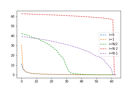
Two things stand out here. First, convergence is much quicker when including the eigenvalues and minors "close" to the eigenvector we are computing. Second, this effect is much greater for the larger eigenvalues. We might recall that for a random matrix, the larger eigenvalues are very spread out. Could this be the reason? We can test this by creating a matrix with evenly spaced eigenvalues, except for the first value which we will keep separated.
a2vals = [x + 2*N for x in lamba]
a2vals[0] = 1
A2 = v.dot(diag(a2vals)).dot(v.T)

relerror0 = compute_converge(A2, a2vals, 0)
# plotting code omitted for brevity
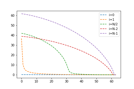
Indeed, with this approach the error is quite low after including the first eigenvalue. Next, let's explore the ordering of the sum. If including the $n$th eigenvalue seems to drop the error the most, what if we added that one first? In fact, let's add minors such that the eigenvalues closest to our target are added first.
def compute_converge2(mat, lamba, i):
    v = zeros((1, mat.shape[1]))
    N = mat.shape[0]
    bottomvals = []
    ratio = zeros((N-1, N))

    order = argsort([abs(lamba[i] - lamba[k]) for k in range(0, N)])[::-1]

    # bottom expression of (1)
    bottom = 1
    for k in order:
        if k == i:
            continue
        bottom *= lamba[i] - lamba[k]
        bottomvals += [bottom]

    for j in order:
        # compute the matrix minor
        ax = list(range(0, j)) + list(range(j+1, N))
        M = mat[:, ax][ax, :]
        lamba_m = eigh(M, eigvals_only=True)

        # top expression of (2)
        top = 1
        for k in range(0, N-1):
            top *= lamba[i] - lamba_m[k]
            ratio[k, j] = top/bottomvals[k]

    # Compute the relative error and return
    relerror = zeros(N)
    for i in range(0, N-1):
        relerror[i] = norm(ratio[-1, :] - ratio[i, :])/norm(ratio[-1, :])

    return relerror
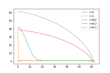
This did seem to improve the convergence for some values, but not the largest eigenvalues. We can leave this to future work, perhaps there is an interesting hint here. Overall, from this method we can see some interesting properties of eigenvectors and eigenvalues, in particular when considering elements local in space or energy.
[1] https://www.quantamagazine.org/neutrinos-lead-to-unexpected-discovery-in-basic-math-20191113/
[2] https://arxiv.org/abs/1908.03795