Exploratory data science on supercomputers for quantum mechanical calculations
I'd like to announce a technical note of ours in Electronic Structure, which highlights some of the Python packages we have been developing to help us perform electronic structure simulations. Python is a really nice glue language that allows you to setup what you want to do, join together multiple programs and methods, and finally analyze your results (statistics, visualizations, etc). It's great to use for science when running Jupyter notebooks: you can interactively build a study which contains all of the steps, decision making processes, and results in one place. Instead of writing throwaway scripts or full fledged software, Jupyter lets you develop and bundle a narrative about what you did, how and why you did it, and what you learned at the end. A lot of these ideas are summed up in the concept of Literate Programming, first introduced by the great computer scientist Donald Knuth in the 1980s.
This style of research is addictive, but you need good, expressive libraries to make sure your notebook doesn't become unwieldy. One of my colleagues said what we need is really something like a Domain Specific Language to succinctly and clearly describe the calculation steps we are doing. Building libraries to help with such intentionality is the theme of our technical note. I will go into the details of one of them below.
Remote Manager and the Coffee Shop Dilemma
Suppose you're sitting in a coffee shop, trying to get some Jupyter based programming done. Suddenly, you get to the part where you need to run some heavy QM calculations. At this point, you have two things you need to be worried about:
- The refill dilemma: the coffee may finish before the calculation does.
- The battery dilemma: your computer's battery may be exhausted before the coffee is finished.
(For my European colleagues, please understand that in other parts of the world we like to leasurely sip a mug of coffee, instead of putting the "Express" in "Espresso").
These problems can in principle be solved by running your calculation on a powerful remote machine. But this requires you to break the notebook workflow. Wouldn't it be nice if Jupyter had the ability to run select parts of your workflow elsewhere?
! pip install -qq remotemanager
This is our remotemanager package. At RIKEN, we have a reasonably powerful supercomputer called Hokusai "Big Waterfall", named after Japan's famous Ukiyo-e artist. When you submit a job on Hokusai, the jobscript looks something like this:
template = """#!/bin/bash
#SBATCH --ntasks-per-node=#MPI#
#SBATCH --cpus-per-task=#OMP#
#SBATCH --nodes=#NODES#
#SBATCH --mem=#MEM:default=112G#
#SBATCH --partition=#QUEUE:default=mpc#
#SBATCH --time=#TIME:format=time:default=3600#
#SBATCH --account=#account#

export OMP_NUM_THREADS=${SLURM_CPUS_PER_TASK}
export BIGDFT_MPIRUN="srun --cpus-per-task=${SLURM_CPUS_PER_TASK}"

# Modules
module load intel
eval "$(~/miniconda3/bin/conda shell.bash hook)" # Miniconda python
conda activate #conda#

# BigDFT Installation Info
export PYTHONPATH=$PYTHONPATH:~/binaries/bdft/install/lib/python3.11/site-packages/
export BIGDFT_ROOT=~/binaries/bdft/install/bin/
"""
We're skipping to the middle of the documentation here, but it's a fine place to start for a blog post. In our template, I've written inside the hashes the things we'd like to modify.
from remotemanager import BaseComputer
url = BaseComputer(template=template,
                   submitter="sbatch", # since it's slurm
                   host="hokusai.riken.jp", # url of hokusai
                   ssh_insert="-q" # this hides the login message
                  )
url.mpi = 16
url.omp = 7
url.nodes = 1
url.conda = "bigdft"
url.account = "RB######"
print(url.script())
1 2 3 4 5 6 7 8 9 10 11 12 13 14 15 16 17 18 19 20 | |
Now let's imagine I want to run a BigDFT calculation in my notebook. I could do this on my current machine, but how much better it would be to do it on Hokusai.
from remotemanager import SanzuFunction
@SanzuFunction(url=url)
def calc_bigdft(geom):
    from BigDFT.Database.Molecules import get_molecule
    from BigDFT.Calculators import SystemCalculator
    from BigDFT.Inputfiles import Inputfile
    calc = SystemCalculator()
    inp = Inputfile()
    inp.set_xc("PBE") ; inp.set_hgrid(0.37)
    log = calc.run(sys=get_molecule(geom), input=inp, name=geom)
    return log.energy
# for demonstration, we don't need so many cores
url.mpi = 1
url.omp = 1
url.mem = "1G"
calc_bigdft("H2O")
appended run runner-0
Running Dataset
assessing run for runner dataset-741a12c3-runner-0... running
Transferring 4 Files... Done
Fetching results
Transferring 1 File... Done

-17.22109431242808
It's just that simple. And don't worry, if you decide to shut down your computer and go to the next shop, these results are cached and immediately available upon notebook restart.
calc_bigdft("H2O")
runner runner-0 already exists
Running Dataset
assessing run for runner dataset-741a12c3-runner-0... ignoring run for successful runner
Fetching results
No Transfer Required

-17.22109431242808
A lot of times I think of a "scaling up" pattern with remotemanager. First I might define a function I want to try and run it on something small. Then as soon as I need to do something heavy, I promote it to a SanzuFunction to run on a more powerful machine.
We have just fetched the energy here. But maybe we'd also like to read the logfile and get out the forces too. We could've used the extra_files_recv option to pull the log back to our local machine. Or we can run another script on the login node and avoid moving files around (some data gets really big).
front_template = """#!/bin/bash
# suppress that this writes to standard error on login nodes
module load intel > /dev/null 2>&1
eval "$(~/miniconda3/bin/conda shell.bash hook)" # Miniconda python
conda activate #conda#
export PYTHONPATH=$PYTHONPATH:~/binaries/bdft/install/lib/python3.11/site-packages/
"""
furl = BaseComputer(template=front_template,
                    host="hokusai.riken.jp", ssh_insert="-q")
furl.conda = "bigdft"
An alternative way to do remote runs is with Jupyter magics.
%load_ext remotemanager
%%sanzu url=furl, asynchronous=False
%%sargs geom="H2O"
from BigDFT.Logfiles import Logfile
log = Logfile(f'log-{geom}.yaml')
log.forces
appended run runner-0
Running Dataset
assessing run for runner dataset-9208d5eb-runner-0... running
Transferring 4 Files... Done
Fetching results
Transferring 1 File... Done

[{'O': [3.388131789017e-21, 4.614988304672e-07, 0.01480963171734]},
 {'H': [-6.617444900424e-24, 0.009705317490556, -0.007404637128436]},
 {'H': [6.617444900424e-24, -0.009705778989387, -0.007404994588901]}]
The asynchronous part here is because Hokusai staff don't like us running background processes on the front end.
Dataset Calculations - Training a Forcefield
Data parallel calculations are another example of the "scaling up" pattern. For this, remotemanager provides the Dataset class. Let's say I want to compute a potential energy surface (following a different BigDFT Tutorial).
from BigDFT.IO import read_pdb
with open("mol.pdb") as ifile:
    sys = read_pdb(ifile)
_ = sys.display()
3Dmol.js failed to load for some reason. Please check your browser console for error messages.
We will rotate on the axis between the two fragments.
from remotemanager import RemoteFunction
# Decorator lets us use this function from any remote calculation
@RemoteFunction
def generate_rotated(geom, angle):
    from BigDFT.IO import read_pdb
    with open(geom + ".pdb") as ifile:
        sys = read_pdb(ifile)
    vec = [x - y for x, y in zip(sys["FRA:0"][0].get_position(),
                                 sys["FRA:1"][0].get_position())]
    sys["FRA:0"].rotate_on_axis(angle=angle, axis=vec, units="degrees")
    return sys
def calc(geom, angle, name):
    from BigDFT.Calculators import SystemCalculator
    from BigDFT.Inputfiles import Inputfile
    calc = SystemCalculator()
    inp = Inputfile()
    inp.set_xc("PBE") ; inp.set_hgrid(0.37)
    log = calc.run(sys=generate_rotated(geom, angle),
                   input=inp, name=name)
    return log.energy
We associate a dataset with the function we just defined.
from remotemanager import Dataset
ds = Dataset(calc, url=url,
             extra_files_send="mol.pdb")
Append each of the runs to the data and run everything.
steps = 11
angles = []
with ds.lazy_append() as la:  # bundling the appends is quicker
    for i in range(steps):
        angles += [120 / (steps - 1) * i]
        la.append_run({"geom": "mol", "angle": angles[-1], "name": f"H2O-{i}"})
ds.run() ; ds.wait() ; ds.fetch_results()
Running Dataset
assessing run for runner dataset-eb87882e-runner-0... running
assessing run for runner dataset-eb87882e-runner-1... running
assessing run for runner dataset-eb87882e-runner-2... running
assessing run for runner dataset-eb87882e-runner-3... running
assessing run for runner dataset-eb87882e-runner-4... running
assessing run for runner dataset-eb87882e-runner-5... running
assessing run for runner dataset-eb87882e-runner-6... running
assessing run for runner dataset-eb87882e-runner-7... running
assessing run for runner dataset-eb87882e-runner-8... running
assessing run for runner dataset-eb87882e-runner-9... running
assessing run for runner dataset-eb87882e-runner-10... running
Transferring 25 Files in 2 Transfers... Done
Fetching results
Transferring 11 Files... Done
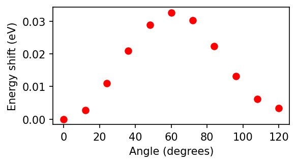
from matplotlib import pyplot as plt
fig, axs = plt.subplots(figsize=(4, 2), dpi=150)
axs.plot(angles, [27.2114 * (x - min(ds.results)) for x in ds.results], 'ro')
axs.set_ylabel("Energy shift (eV)")
_ = axs.set_xlabel("Angle (degrees)")
From Data to Machine Learning
One of my motivations for this blog post was to test out a machine learning descriptors inside DScribe. First, create the descriptors.
from BigDFT.Interop.ASEInterop import bigdft_to_ase
structures = []
for i in range(steps):
    structures += [bigdft_to_ase(generate_rotated("mol", angles[i]))]
from dscribe.descriptors import SOAP
soap = SOAP(species=set([x.sym for x in sys.get_atoms()]), periodic=False,
            r_cut=5.0, n_max=8, l_max=8)
X = [soap.create(s).flatten() for s in structures]
We will try linear regression as our model (since this is linear regression, we can stick to the local machine).
from sklearn.linear_model import LinearRegression
model = LinearRegression()
_ = model.fit(X, ds.results)
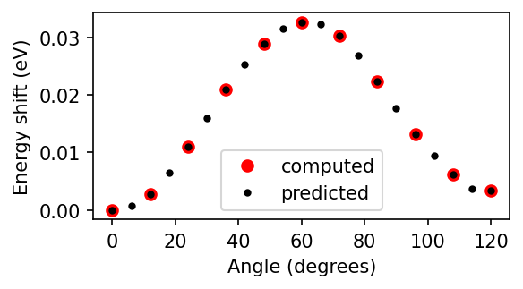
Now predict some additional values.
steps = (steps - 1) * 2 + 1
pstructures = []
pangles = []
for i in range(steps):
    pangles += [120 / (steps - 1) * i]
    pstructures += [bigdft_to_ase(generate_rotated("mol", pangles[-1]))]
X = [soap.create(s).flatten() for s in pstructures]
predictions = model.predict(X)
fig, axs = plt.subplots(figsize=(4, 2), dpi=150)
axs.plot(angles, [27.2114 * (x - min(ds.results)) for x in ds.results],
         'ro', label="computed")
axs.plot(pangles, [27.2114 * (x - min(ds.results)) for x in predictions],
         'k.', label="predicted")
axs.set_ylabel("Energy shift (eV)")
axs.set_xlabel("Angle (degrees)")
_ = axs.legend()
You could imagine that as the machine learning part gets more heavy, you move that to the remote machine as well thanks to remotemanager.