Lennard Jones Potential
The Lennard-Jones potential is a well studied model potential. It has a very simple form: $$V(r) = 4\epsilon \bigg[ \big(\frac{\sigma}{r}\big)^{12} - \big(\frac{\sigma}{r}\big)^{6} \bigg].$$ In order to use this potential, you need to know what your two parameters $\epsilon$ and $\sigma$ are. In this post, I thought it would be fun try to extract those parameters from quantum chemistry calculations, and see how good of a job it does.
from matplotlib import rcParams
from matplotlib import pyplot as plt
rcParams['axes.labelsize'] = 14
rcParams['xtick.labelsize'] = 12
rcParams['ytick.labelsize'] = 12
rcParams['legend.fontsize'] = 12
rcParams["lines.linewidth"] = 3
rcParams["lines.markersize"] = 12
rcParams["axes.formatter.useoffset"] = False
rcParams["axes.formatter.limits"] = [-2, 5]
First, let's pick some atomic elements to compute. We'll pick some noble gases as typical Lennard-Jones systems.
elements = [("He", "He"), ("Ne", "Ne"), ("He", "Ne"), ("Ar", "Ne")]
We will use a dictionary to store each dimer as two fragments. Note that we start with the atoms overlapping because we're going to vary the distance later.
dimers = {}
for e in elements:
    dimers[e] = {}
    dimers[e]["FRA:0"] = [[e[0], 0, 0, 0]]
    dimers[e]["FRA:1"] = [[e[1], 0, 0, 0]]
The next step is to define a function which computes the interaction energy between two molecules. We will use PySCF to compute energies at the MP2//cc-pVDZ level of theory. Ideally we'd use a higher level of theory, but for the purposes of this blog post we'll just stick with MP2 and a smaller basis.
def get_energy(istr):
    from pyscf import M, cc
    mol = M(atom=istr, basis='ccpvdz')
    hf = mol.HF().run(verbose=False)
    mp = hf.MP2().run(verbose=False)
    return mp.e_tot
def quan_ene(d, dim):
    istr = ""
    for at in dim["FRA:0"]:
        istr += " ".join([str(x) for x in at]) + ";"
    mon_ene = get_energy(istr)

    istr2 = ""
    for at in dim["FRA:1"]: # this loop includes the distance shift
        istr2 += " ".join([str(x) for x in at[:-1]]) + " " + str(at[-1] + d) + ";"
    mon_ene += get_energy(istr2)

    dim_ene = get_energy(istr + ";" + istr2)

    return dim_ene - mon_ene
How do we extract the parameters now? One option we have is to use the curve fitting feature to try and match the function. There is a simpler approach though, using a bit of calculus. First, define the Lennard-Jones potential using sympy.
from sympy.abc import r
from sympy.physics.units.quantities import Quantity
epsilon = Quantity("ε")
sigma = Quantity("σ")
lj = 4 * epsilon * ((sigma/r)**12 - (sigma/r)**6)
lj
$$\displaystyle 4 \left(\frac{\text{σ}^{12}}{r^{12}} - \frac{\text{σ}^{6}}{r^{6}}\right) \text{ε}$$
Now we can compute the minimum of this function on the domain of positive reals.
from sympy import diff
from sympy.solvers.solveset import solveset_real
dlj = diff(lj, r)
extrema = [x for x in solveset_real(dlj, r) if x > 0][0]
extrema
$$\displaystyle \sqrt[6]{2} \text{σ}$$
Last the value of the function at this minimum point.
lj.subs('r', extrema)
$$\displaystyle - \text{ε}$$
We thus can discover that the Lennard-Jones potential has its minimum at distance $r = 2^{\frac{1}{6}}\sigma$ with value $V(r) = -\epsilon$. That means to get these parameters we simply have to find the interatomic distance of the minimum energy value of our system. We could of course perform geometry optimization, but in this case of symmetric atoms in 1D it's simple enough to just use a black box minimizer.
from scipy.optimize import minimize

opt_result = {}
for e in elements:
    opt_result[(e[0],e[1])] = minimize(fun=lambda x: quan_ene(x[0], dimers[e]), x0=2)
    opt_result[(e[1],e[0])] = opt_result[(e[0],e[1])]
In order to compare and plot the results, we can also compute the values on a distance grid.
from numpy import linspace
energies = {}

for e in elements:
    energies[e] = {}
    grid = linspace(opt_result[e].x[0] - 0.5, 8, 100)
    for d in grid:
        energies[e][d] = quan_ene(d, dimers[e])
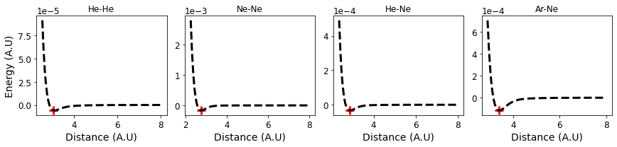
Below we will plot the values on the grid as well as the minimum value to verify the optimization procedure.
fig, axs = plt.subplots(1,len(elements),figsize=(12,3))

for i, e in enumerate(elements):
    axs[i].plot(list(energies[e]), list(energies[e].values()),
                linestyle='--', color='k')
    axs[i].set_xlabel("Distance (A.U)")
    axs[i].set_title("-".join(e))
    axs[i].scatter(opt_result[(e)].x, opt_result[(e)].fun, marker='+', color='r')
axs[0].set_ylabel("Energy (A.U)")
fig.tight_layout()
With the Lennard-Jones parameters computed, we can now turn to computing the actual function.
def lennard_jones(r, epsilon, sigma):
    return 4 * epsilon * ((sigma/r)**12 - (sigma/r)**6)
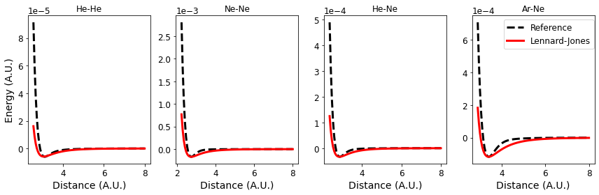
We can plot both the reference values and those values computed with the potential on the same grid to see how this potential does.
from matplotlib import pyplot as plt
fig, axs = plt.subplots(1, len(elements), figsize=(12, 4))

for i, e in enumerate(elements):
    xvals = list(energies[e])

    scale = 2**(1/6.0)
    computed = [lennard_jones(x, -1*opt_result[(e)].fun,
                              opt_result[(e)].x[0]/scale) for x in xvals]

    axs[i].plot(xvals, list(energies[e].values()),
                linestyle='--', color='k', label="Reference")
    axs[i].plot(xvals, computed,
                linestyle='-', color='r', label="Lennard-Jones")
    axs[i].set_xlabel("Distance (A.U.)")
    axs[i].set_title("-".join(e))

axs[-1].legend(bbox_to_anchor=[1.03,1.])
axs[0].set_ylabel("Energy (A.U.)")
fig.tight_layout()
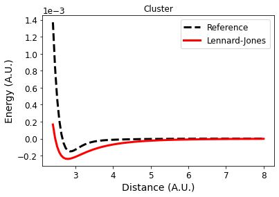
Now let's consider a system with more than two atoms of different types. In this case, we might hope that the interactions we parameterized can be additive. Let's test this out.
def lennard_jones_group(dim, dist):
    from numpy import array
    from numpy.linalg import norm
    etot = 0
    for at1 in dim["FRA:0"]:
        for at2 in dim["FRA:1"]:
            key = (at1[0], at2[0])
            epsilon = opt_result[key].fun
            sigma = opt_result[key].x[0]/2**(1/6.0)

            shifted = at2[1:]
            shifted[-1] += dist

            r = norm(array(at1[1:]) - shifted)
            etot += -4 * epsilon * ((sigma/r)**12 - (sigma/r)**6)
    return etot
Our test cluster will be two squares of He and Ne atoms.
cluster = {}
cluster["FRA:0"] = [["He", 0, 0, 0], ["Ne", 3, 0, 0], ["He", 0, 3, 0], ["Ne", 3, 3, 0]]
cluster["FRA:1"] = [["He", 3, 0, 0], ["Ne", 0, 0, 0], ["He", 3, 3, 0], ["Ne", 0, 3, 0]]
Compute the reference values on a grid.
grid = linspace(2.4, 8, 100)
energies["cluster"] = {}
for d in grid:
    energies["cluster"][d] = quan_ene(d, cluster)
Plot.
fig, axs = plt.subplots(1, 1)
xvals = list(energies[("cluster")])
computed = [lennard_jones_group(cluster, x) for x in xvals]

axs.plot(xvals, list(energies[("cluster")].values()),
         linestyle='--', color='k', label="Reference")
axs.plot(xvals, computed,
         linestyle='-', color='r', label="Lennard-Jones")
axs.set_xlabel("Distance (A.U.)")
axs.set_title("Cluster")
axs.set_ylabel("Energy (A.U.)")
axs.legend()
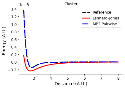
What is the source of the error in this case? It can either be from our two body pairwise approximation or from the accumulation of errors from the inexact Lennard-Jones potential. To tease that out, let's also plot the energy that comes from doing MP2 in a pairwise way.
def pairwise_mp2(d, dim):
    etot = 0
    for at1 in dim["FRA:0"]:
        at1str = " ".join([str(x) for x in at1])+";"
        mon_ene = get_energy(at1str)
        for at2 in dim["FRA:1"]:
            at2str = " ".join([str(x) for x in at2[:-1]]) + " " + str(at2[-1] + d) + ";"
            mon_ene2 = get_energy(at2str)

            dim_ene = get_energy(at1str + ";" + at2str)
            etot += dim_ene - (mon_ene + mon_ene2)
    return etot
grid = linspace(2.4, 8, 100)
energies["pairwise_cluster"] = {}
for d in grid:
    energies["pairwise_cluster"][d] = pairwise_mp2(d, cluster)
fig, axs = plt.subplots(1,1)
xvals = list(energies[("cluster")])
computed = [lennard_jones_group(cluster, x) for x in xvals]

axs.plot(xvals, list(energies[("cluster")].values()),
         linestyle='--', color='k', label="Reference")
axs.plot(xvals, computed,
         linestyle='-', color='r', label="Lennard-Jones")
axs.plot(xvals, list(energies[("pairwise_cluster")].values()),
         linestyle='-.', color='b', label="MP2 Pairwise")
axs.set_xlabel("Distance (A.U.)")
axs.set_title("Cluster")
axs.set_ylabel("Energy (A.U.)")
axs.legend()