Probing Disorder in 2CzPN using Core and Valence States
I want to share a new paper I worked on with Dr. Laura Ratcliff of the University of Bristol called Probing Disorder in 2CzPN using Core and Valence States. In this paper, we explored a molecular called 2CzPN which is of interest for devices based on Thermally Activated Delayed Fluorescence.
I wanted to use this occasion to mention that I'm trying to package up PyBigDFT for distribution. It can be pip installed right now using these commands:
! pip install -q pyFutile
! pip install -q PyBigDFT
Another option is to install the whole BigDFT suite using conda (linux only unfortunately):
! conda install -c conda-forge bigdft-suite
We can take a look at the 2CzPN molecule with the help of PyBigDFT. 2CzPN is available on pubchem with the following canonical smiles.
smi = "C1=CC=C2C(=C1)C3=CC=CC=C3N2C4=C(C=C(C(=C4)C#N)C#N)N5C6=CC=CC=C6C7=CC=CC=C75"
We can generate the 3d version using openbabel. In fact, I've wrapped up this process in PyBigDFT.
from BigDFT.Interop.BabelInterop import build_from_smiles
mol = build_from_smiles(smi, form="can")
By default, this constructs a system composed of a single fragment. But for our purposes I'd like to split it up into atoms.
from BigDFT.Systems import System, copy_bonding_information
from BigDFT.Fragments import Fragment
atsys = System()
for i, at in enumerate(mol["UNL1:1"]):
atsys["FRA:"+str(i)] = Fragment([at])
copy_bonding_information(mol, atsys)
Let's see how it looks using py3Dmol.
from BigDFT.Visualization import InlineVisualizer, get_atomic_colordict
viz = InlineVisualizer()
viz.display_system(atsys, colordict=get_atomic_colordict(atsys))
You appear to be running in JupyterLab (or JavaScript failed to load for some other reason). You need to install the 3dmol extension:
jupyter labextension install jupyterlab_3dmol
Fragmentation
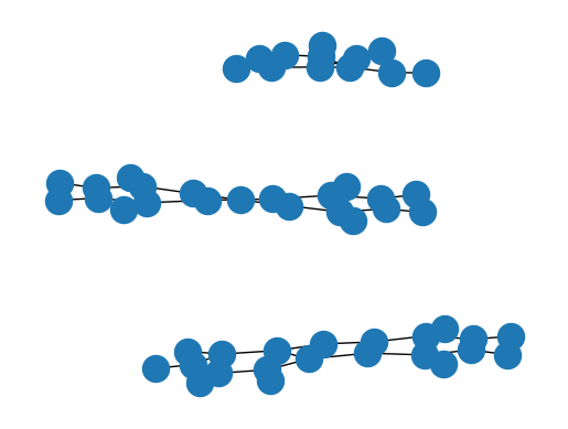
When I look at this system, I think of it as being broken up into three parts: the body and two wings. Indeed the C-N bonds connecting the body to the wings are quite ammenable to rotation. Let's split up the system into fragments defined by these parts. This is not a trivial task, though maybe some software that is smart about romotomers could do it (openbabel failed...). It's also something you could do by hand without too much trouble. But we will do it the fun way.
Each system has a connectivity matrix associated with it:
# Links to/from fragment 2, atom 0
print(atsys.conmat["FRA:2"][0])
{('FRA:1', 0): 1, ('FRA:3', 0): 1, ('FRA:38', 0): 1.0}
We need to remove the bonds that connect the different parts. First, we find the nitrogens that are bonded to three carbons. That will give us 2x3 different candidate links to cut.
candidates = []
nitrogens = []
for fragid, frag in atsys.items():
for i, at in enumerate(frag):
# Find the nitrogen which is bonded to three different atoms
if at.sym != "N":
continue
links = atsys.conmat[fragid][i]
if len(links) != 3:
continue
nitrogens.append(fragid)
candidates.extend(list(links))
print(nitrogens)
print(candidates)
['FRA:12', 'FRA:23']
[('FRA:11', 0), ('FRA:3', 0), ('FRA:13', 0), ('FRA:14', 0), ('FRA:24', 0), ('FRA:35', 0)]
The two candidate carbons that are bonded to each other are the ones we are after.
cuts = []
for fragid, _ in candidates:
links = atsys.conmat[fragid][0]
if any([x in candidates for x in links]):
cuts.append(fragid)
print(cuts)
['FRA:13', 'FRA:14']
Remove those links from the connectivity matrix.
from copy import deepcopy
cutsys = deepcopy(atsys)
for n in nitrogens:
for c in cuts:
cutsys.conmat[n][0].pop((c, 0), None)
cutsys.conmat[c][0].pop((n, 0), None)
Now that we've made those cuts, we know that the three fragments can be defined by the sets of atoms which can reach each other by walking along the connectivity matrix. The networkx package can simplify this work considerably.
from networkx import Graph
g = Graph()
for fragid, frag in cutsys.items():
for i, at in enumerate(frag):
g.add_node((fragid, i))
for fragid1, frag in cutsys.conmat.items():
for i, at in enumerate(frag):
for fragid2, j in at:
g.add_edge((fragid1, i), (fragid2, j))
from networkx import draw, spring_layout
from matplotlib import pyplot as plt
fig, ax = plt.subplots()
draw(g, ax=ax, pos=spring_layout(g, iterations=100, seed=0))
The conversion appears to have worked. Now we use networkx's facility for subgraph iteration and generate the new fragments.
from networkx import connected_components
splitsys = System({"BOD:0": Fragment(),
"WNG:1": Fragment(),
"WNG:2": Fragment()})
for i, sg in enumerate(sorted(connected_components(g), key=len)):
if i == 0:
fid = "BOD"
else:
fid = "WNG"
for n in sg:
splitsys[fid + ":"+str(i)].append(cutsys[n[0]][n[1]])
copy_bonding_information(mol, splitsys)
_ = splitsys.display()
You appear to be running in JupyterLab (or JavaScript failed to load for some other reason). You need to install the 3dmol extension:
jupyter labextension install jupyterlab_3dmol
Manipulation
The next step is to try rotating one of the wings, and see how that affects the system. Again, we have to search for the link between the body and a wing.
for i, _ in enumerate(splitsys["BOD:0"]):
for link in splitsys.conmat["BOD:0"][i]:
if link[0] == "WNG:1":
atm1 = ("BOD:0", i)
atm2 = link
break
print(atm1, atm2)
('BOD:0', 3) ('WNG:1', 13)
Now create the rotated systems.
# Rotate along the axis defined by the bond, centered at the connecting atom
cent = splitsys[atm1[0]][atm1[1]].get_position()
axis = [x - y for x, y in zip(splitsys[atm2[0]][atm2[1]].get_position(), cent)]
from numpy import linspace
systems = {}
for ang in linspace(-30, 30, 9):
systems[ang] = deepcopy(splitsys)
systems[ang]["WNG:1"].rotate_on_axis(ang, axis=axis, centroid=cent, units="degrees")
viz = InlineVisualizer()
for sys in systems.values():
viz.display_system(sys, show=False)
viz.display_system(splitsys)
You appear to be running in JupyterLab (or JavaScript failed to load for some other reason). You need to install the 3dmol extension:
jupyter labextension install jupyterlab_3dmol
Calculation
Now we have a list of systems with different angles. To keep things light, we can use XTB for the calculations.
from BigDFT.Interop.XTBInterop import XTBCalculator
code = XTBCalculator(skip=True, verbose=False)
logfiles = {}
for ang, sys in systems.items():
logfiles[ang] = code.run(sys=sys, name=str(ang), run_dir="scr")
Extract the energy and gaps.
energies = {k: v.energy for k, v in logfiles.items()}
gaps = {}
for ang, log in logfiles.items():
for line in log.log.split("\n"):
if "HL-Gap" in line:
gaps[ang] = float(line.split()[3])
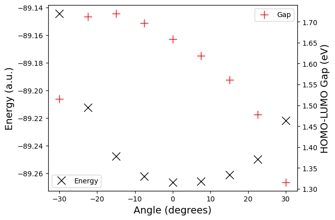
Plot.
fig, axs = plt.subplots(1, 1)
axs.plot(list(systems), [energies[x] for x in systems],
'kx', markersize=12, label="Energy")
axs2 = axs.twinx()
axs2.plot(list(systems), [gaps[x] for x in systems],
'r+', markersize=12, label="Gap")
axs.set_ylabel("Energy (a.u.)", fontsize=14)
axs2.set_ylabel("HOMO-LUMO Gap (eV)", fontsize=14)
axs.set_xlabel("Angle (degrees)", fontsize=14)
axs.legend(loc="lower left")
axs2.legend()
pass
As you can see, PyBigDFT wraps up a lot of my favorite python libraries. This notebook revealed the further utility of networkx, which I think deserves its own interperability module in the near future.