Probing the mutational landscape of the SARS-CoV-2 spike protein via quantum mechanical modeling of crystallographic structures

Sat 31 December 2022 in Lessons

#publication

Two straight blog posts based on "Probing" I guess. This time I want to announce a paper called Probing the mutational landscape of the SARS-CoV-2 spike protein via quantum mechanical modeling of crystallographic structures. In this work, we wanted to study the different variants of SARS-CoV-2. We did this by studying how the different mutations impact binding of the spike protein. All calculations were done with BigDFT and using our complexity reduction framework, which meant we could use quantum mechanical calculations for unique insight into the evolutionary process.

With that paper finished, I thought it would be fun to make a simple workflow that plays with the tools we used in this study.

PDBFixer and In-Silico Mutations

A really nice tool for these kind of studies is PDBFixer. Our focus is on crystal structures, and many of them exist in the RCSB Database. However, these structures cannot be treated as is, and instead require some prep work such as fixing missing residues, adding hydrogen atoms, etc. PDBFixer is one tool that can help with this. For example, let's fetch a small protein called 5awl.

! pdbfixer --pdbid=5awl --output=5awl.pdb --add-atoms="none" --keep-heterogens=none

! head 5awl.pdb

REMARK   1 PDBFIXER FROM: http://www.rcsb.org/pdb/files/5awl.pdb
REMARK   1 CREATED WITH OPENMM 7.7, 2023-01-04
CRYST1   19.246   33.597   11.551  90.00  90.00  90.00 P 1           1 
ATOM      1  N   TYR A   1      25.824  21.671  10.238  1.00  0.00           N  
ATOM      2  CA  TYR A   1      24.935  20.652  10.774  1.00  0.00           C  
ATOM      3  C   TYR A   1      23.729  20.558   9.852  1.00  0.00           C  
ATOM      4  O   TYR A   1      23.390  21.602   9.289  1.00  0.00           O  
ATOM      5  CB  TYR A   1      24.425  21.029  12.167  1.00  0.00           C  
ATOM      6  CG  TYR A   1      25.525  21.526  13.070  1.00  0.00           C  
ATOM      7  CD1 TYR A   1      25.829  22.870  13.275  1.00  0.00           C

It's also possible to use PDBFixer through its python API. PDBFixer is related to openmm so it has a lot of features.

from pdbfixer import PDBFixer
fixer = PDBFixer(filename='5awl.pdb')

# Build a list of residues while we're at it
rlist = []
print("Residues:")
for res in fixer.topology.residues():
    print("\t -", res.name, res.id)
    rlist.append((res.name, res.id))

print("Chains:")
for chain in fixer.topology.chains():
    print("\t -", chain.id)

Residues:
     - TYR 1
     - TYR 2
     - ASP 3
     - PRO 4
     - GLU 5
     - THR 6
     - GLY 7
     - THR 8
     - TRP 9
     - TYR 10
Chains:
     - A

This is the setup we need if we want to start mutating our system. We create a list of mutations to apply, which are named after the residues and IDs. For example, mutation Gly5 -> Arg

from copy import deepcopy
mutations = ["GLU-5-ARG"]
mutated = deepcopy(fixer)
mutated.applyMutations(mutations, "A")
mutated.findMissingResidues()  # Needed even if there are none.
mutated.findMissingAtoms()
mutated.addMissingAtoms()
mutated.addMissingHydrogens(7.0)
for res in mutated.topology.residues():
    print("-", res.name, res.id)

- TYR 1
- TYR 2
- ASP 3
- PRO 4
- ARG 5
- THR 6
- GLY 7
- THR 8
- TRP 9
- TYR 10

Mutation Generation

It could be interesting to use this feature to try out a large library of mutations. A PAM Matrix is a matrix which describes the probability of various point mutations occuring in nature. One such matrix is called PAM250, and you can download it it from NIH.

! wget https://ftp.ncbi.nih.gov/blast/matrices/PAM250

We can process it in fairly simply.

freq = {}
with open("PAM250") as ifile:
    line = next(ifile)
    while "#" in line:
        line = next(ifile)
    order = line.split()
    for line in ifile:
        split = line.split()
        k1 = split[0]
        freq[k1] = {}
        for k2, v in zip(order, split[1:]):
            freq[k1][k2] = float(v)

These are log probabilities based on the letter representations of amino acids.

print(freq["A"]["C"])

-2.0

The only problem is that the letter codes are not compatability with our API. Fortunately BioPython has a utility for this.

from Bio.PDB.Polypeptide import one_to_three
print(one_to_three("W"))

TRP

Let's convert our dictionary. At the same time, we'll toss out the non-standard stuff.

freqn = {}
for k1, inner in freq.items():
    try:
        n1 = one_to_three(k1)
    except KeyError:
        continue
    freqn[n1] = {}
    for k2, v in inner.items():
        try:
            n2 = one_to_three(k2)
        except KeyError:
            continue
        freqn[n1][n2] = v

print(freqn["ALA"]["CYS"])

-2.0

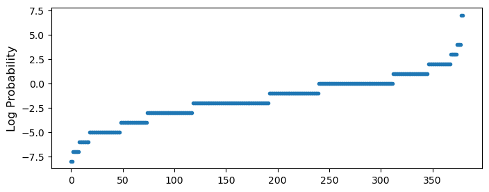
It is interesting to look at the distribution of off diagonal values.

from matplotlib import pyplot as plt
vals = []
for k1, inn in freqn.items():
    for k2, v in inn.items():
        if k1 == k2:
            continue
        if v > 6:
            print(k1, k2)
        vals.append(v)
fig, axs = plt.subplots(1, 1, figsize=(8,3))
axs.plot(sorted(vals), '.')
_ = axs.set_ylabel("Log Probability", fontsize=12)

PHE TYR
TYR PHE

Distribution

Sampling

Time to generate a bunch of mutations. Basically, what I wanted to do was just go into a loop, generate a random mutation, roll the dice to see if we should accept it, and if so add it to the list. But that is a major pain with this distribution since we'd need to sample a huge number of times to find something valid. Primarily the pain comes from mutations Phe->Tyr and back, which are the two outliers on the far right. For this notebook, we'll clip the probablity, essentially, by maxing our random numbers at $10^4$ to speed things up.

from random import seed, sample, uniform
seed(0)
mutations = []
while len(mutations) < 20:
    # Get a residue in the middle of the protein (not first or last)
    amn1, idx1 = sample(rlist[1:-1], 1)[0]
    # Get something random to change it to
    amn2 = sample(list(freqn), 1)[0]
    # Remove do nothing
    if amn1 == amn2:
        continue
    # Form the mutation string
    mstr = amn1 + "-" + str(idx1) + "-" + amn2
    if mstr in mutations:
        continue
    # Roll the dice, and see if the mutation should be accepted
    odds = uniform(1e-8, 1e4)
    if 10**freqn[amn1][amn2] > odds:
        mutations.append(mstr)

Add a base mutation where nothing happens.

bname = rlist[0][0] + "-" + str(rlist[0][1]) + "-" + rlist[0][0]
mutations = [bname] + mutations

The new structures can be generated and saved to disk.

from os import mkdir
try:
    mkdir("structs")
except:
    pass

from openmm.app import PDBFile
from os.path import join

for m in mutations:
    msys = deepcopy(fixer)
    msys.applyMutations([m], "A")
    msys.findMissingResidues()
    msys.findMissingAtoms()
    msys.addMissingAtoms()
    msys.addMissingHydrogens(7.0)
    with open(join("structs", m + ".pdb"), "w") as ofile:
        PDBFile.writeFile(msys.topology, msys.positions, ofile)

Mutation Evaluation

How do we evaluate the structures we generated? Something simple we might investigate is how soluable they are in water. For this, we can perform a geometry optimization and single point energy calculation using XTB's GFN-FF, and extract the solvation energy.

from BigDFT.Interop.XTBInterop import XTBCalculator
calc = XTBCalculator(skip=True, verbose=False)

from BigDFT.IO import read_pdb
from BigDFT.UnitCells import UnitCell

energies = {}
for m in mutations:
    with open(join("structs", m + ".pdb")) as ifile:
        sys = read_pdb(ifile)
    sys.cell = UnitCell()  # Free boundary

    # Get the net charge of the system. This will work for our 
    # simple system, but not in general!
    charge = 0
    for fragid in sys:
        fname = fragid.split(":")[0]
        if fname in ["ARG", "LYS"]:
            charge += 1
        elif fname in ["ASP", "GLU"]:
            charge -= 1

    # Run the calculation. We need FIRE for optimization to fix
    # some of these ugly mutated residues.
    inp = {}
    inp["opt"] = {"engine": "inertial"}
    log = calc.run(sys=sys, name=m, opt=True, gfnff=True,
                   inp=inp, alpb="water", chrg=charge, run_dir="work")

    # Get the solvation energy, keep looping to the last
    for line in log.log.split("\n"):
        if "-> Gsolv" in line:
            energies[m] = 630*float(line.split()[3])

Visualize the results.

fig, axs = plt.subplots(1, 1, figsize=(8, 3))
axs.plot(list(energies.values()), 'kx', markersize=14)
axs.set_ylabel("Solvation Energy (kcal/mol)", fontsize=12)
axs.set_xlabel("Mutation", fontsize=14)
axs.set_xticks(range(len(list(mutations))))
_ = axs.set_xticklabels(list(mutations), rotation=90)

Mutation Scores

The baseline is the entry on the far left (TYR-1-TYR). Indeed the solvation energy is affected by various mutations. Negatively charged amino acids improve solubility (GLY-7-ASP); don't get rid of them (GLU-5-HIS). The smaller improvements such as PRO-4-ASN are maybe the more interesting results. Overall, PDBFixer makes it very easy for us to modify the amino-acid sequence of proteins, so I recommend you give it a try.