Scipy Optimization for Chemistry
PSI-K Conference
Last month I participated in the PSI-K 2022 Conferece. It was great to travel outside of Japan after three years of COVID-19 restrictions. I got some pretty neat goodies while there:

in addition to enjoying the great Swiss summer weather. Some of the talks got me thinking about optimization, which I thought I'd explore in this notebook.
Optimization
In this post, I want to see how useful the built in scipy optimizers are for quantum chemistry calculations. We'll employ them as black boxes for computing various properties. We will use PySCF as our QM driver and Benzene as a reference molecule.
h_to_eV = 27.2114
!cat Benzene.xyz
12

C         -1.21310       -0.68840        0.00000
C         -1.20280        0.70640        0.00010
C         -0.01030       -1.39480        0.00000
C          0.01040        1.39480       -0.00010
C          1.20280       -0.70630        0.00000
C          1.21310        0.68840        0.00000
H         -2.15770       -1.22440        0.00000
H         -2.13930        1.25640        0.00010
H         -0.01840       -2.48090       -0.00010
H          0.01840        2.48080        0.00000
H          2.13940       -1.25630        0.00010
H          2.15770        1.22450        0.00000
I had some strange issues with PySCF's xyz reader (maybe a buggy version), so I read the molecule in manually.
def read_geom(iname):
    atom = []
    with open(iname) as ifile:
        next(ifile)
        next(ifile)
        for line in ifile:
            split = line.split()
            atom.append([split[0], [float(x) for x in split[1:]]])
    return atom
And build.
from pyscf import gto
mol = gto.Mole()
mol.basis = "6-31G*"
mol.atom = read_geom("Benzene.xyz")
mol.verbose = 0
_ = mol.build()
Example 1: Functional Optimization
As a first example, let's try optimizing the ratio of exact exchange in the PBE0 functional for a given molecule. The goal will be to match the homo-lumo gap of a system. First, we need a reference value, for which we will use $\Delta$SCF.
cat = mol.copy()
cat.charge = 1
cat.spin = 1
_ = cat.build()
from pyscf import dft
mf = dft.RKS(mol)
mf.xc = "PBE0"
ene = mf.kernel()

mf_cat = dft.RKS(cat)
mf_cat.xc = "PBE0"
ene_cat = mf_cat.kernel()
And so the target homo-lumo band gap is:
target_gap = ene_cat - ene
print(target_gap * h_to_eV, "eV")
9.143932978023763 eV
But simply using Koopman's theorem we would haven found a value of
hidx = int(mol.nelec[0])
print(h_to_eV * (mf.mo_energy[hidx] - mf.mo_energy[hidx-1]), "eV")
7.237101946475208 eV
We can write a function which returns the error of computing the gap with Koopman's theorem using given a fixed amount of exchange.
tested_x = []
tested_y = []
def f(mix):
    # Use the LIBXC Codes for PBE_X and PBE_C
    mf.xc = str(mix) + " * HF + " + str(1.0-mix) + " * 101 + 130"
    _ = mf.kernel()
    gap = mf.mo_energy[hidx] - mf.mo_energy[hidx-1]
    err = abs(gap - target_gap) * h_to_eV
    tested_x.append(mix)
    tested_y.append(err)
    return err
print(f(0.25))
1.9068310315485535
Scipy has an optimizer which seems specialized for a single variable, so let's give it a spin.
from scipy.optimize import minimize_scalar
opt = minimize_scalar(f, bounds=(0., 1.), tol=1e-1)
from matplotlib import pyplot as plt
fig, axs = plt.subplots(1, 1, figsize=(4,3))

axs.plot(tested_x, tested_y, 'kx')
axs.axvline(opt.x, color='r', linestyle='--')

axs.set_ylabel("Error (eV)", fontsize=12)
_ = axs.set_xlabel("Ratio", fontsize=12)
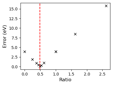
And it looks like the winner is the classic half and half mix. It is a shame that the bounds are violated so severely though, but for it worked for our purposes.
Example 2: Geometry Optimization
As a second example, we will try performing some geometry optimization. Note that PySCF has some extra features for geometry optimization, in particular the scanner mode. But we will do things manually for illustration purposes. We will also use a smaller basis set just to keep the notebook run-time manageable.
mol = gto.Mole()
mol.basis = "STO-3G"
mol.atom = read_geom("Benzene.xyz")
mol.verbose = 0
_ = mol.build()
class OptTarget:
    def __init__(self, mol):
        self.mol = mol.copy()
        self.energies = []  # Store computed energies

    def __call__(self, pos):
        nat = len(self.mol.atom)

        # Reshape the position variable to a per atom
        rpos = pos.reshape(nat, 3)

        # Update the positions
        for i in range(nat):
            self.mol.atom[i][1] = rpos[i]
        self.mol.build()

        # Compute the energy
        mf = dft.RKS(self.mol)
        mf.xc = "PBE0"
        e = mf.kernel()
        self.energies.append(e)

        return e
from scipy.optimize import minimize
t = OptTarget(mol)
opt = minimize(t, x0=mol.atom_coords(), method="CG", tol=1e-2)
fig, axs = plt.subplots(figsize=(4,3))
axs.plot(t.energies, 'kx--')
axs.set_ylabel("Energy (a.u.)", fontsize=12)
axs.set_xlabel("Iteration", fontsize=12)
_ = axs.set_ylim(-229.5, -226)
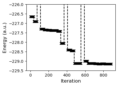
With this basic approach the progress is quite slow. This is because the black box minimizer is trying to numerically approximate the gradient. Since we can get the gradient from the pyscf calculation, let's integrate it into the process.
from pyscf import grad
class OptTarget:
    def __init__(self, mol):
        self.mol = mol.copy()
        self.energies = []  # Store the computed energies
        self.grad_norm = []  # Store the norm of the computed gradients

    def __call__(self, pos):
        from numpy.linalg import norm
        nat = len(self.mol.atom)

        # Reshape the position variable to a per atom
        rpos = pos.reshape(nat, 3)

        # Update the positions
        for i in range(nat):
            self.mol.atom[i][1] = rpos[i]
        self.mol.build()

        # Compute the energy
        mf = dft.RKS(self.mol)
        mf.xc = "PBE0"
        e = mf.kernel()
        self.energies.append(e)

        # Compute the gradient
        mf = grad.RKS(mf)
        g = mf.kernel()
        self.grad_norm.append(norm(g))
        return e, g.flatten()
from scipy.optimize import minimize
t = OptTarget(mol)
opt = minimize(t, x0=mol.atom_coords(), method="CG", jac=True, tol=1e-2)
fig, axs = plt.subplots(figsize=(4,3))
axs.plot(t.energies, 'kx--', label="Energy")
axs.set_ylabel("Energy (a.u.)", fontsize=12)
axs.set_xlabel("Iteration", fontsize=12)
axs.set_ylim(-229.5, -226)
axs.legend(loc="upper left")

axs2 = axs.twinx()
axs2.plot(t.grad_norm, 'r+--', label="Force")
axs2.set_ylabel("Gradient Norm (Å)")
axs2.set_yscale("log")
_ = axs2.legend(loc="upper right")
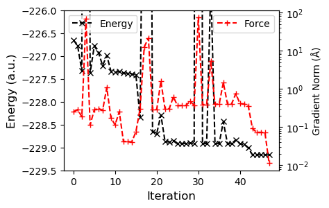
Using the gradient information, convergence is much quicker.
Example 3: Contraction Coefficient Optimization
Now let's try something really fancy: optimization of the contraction coefficients of our basis set.
class OptTarget:
    def __init__(self, mol):
        self.mol = mol.copy()
        self.energies = []  # Store the computed energies

    def __call__(self, coefficients):
        # Build the basis
        basis = {"H": gto.basis.load("STO-3G", "H"),
                 "C": gto.basis.load("STO-3G", "C")}

        # Update with the new coefficients
        i = 0
        for at in basis.values():
            for shell in at:
                for coeff in shell[1:]:
                    coeff[1] = coefficients[i]
                    i += 1
        self.mol.basis = basis
        self.mol.build()

        # Compute the energy
        mf = dft.RKS(self.mol)
        mf.xc = "PBE0"
        e = mf.kernel()
        self.energies.append(e)

        return e
I'll manually write the starting coefficients of the STO-3G basis set as our initial guess.
t = OptTarget(mol)
start_coeff = [0.1543289673E+00,  0.5353281423E+00, 0.4446345422E+00, #H 1S
               0.1543289673E+00,  0.5353281423E+00, 0.4446345422E+00, #C 1S
               -0.9996722919E-01, 0.3995128261E+00, 0.7001154689E+00, #C 2S
               0.1559162750E+00,  0.6076837186E+00, 0.3919573931E+00] #C 2p
Optimize and plot. This time the TNC method is used because we are constraining the contraction coefficients to be between -1 and 1. In practice we probably would want to impose more sophisticated constraints.
opt = minimize(t, x0=start_coeff, bounds=[(-1, 1) for _ in start_coeff],
               method="TNC", tol=1e-2)
fig, axs = plt.subplots(figsize=(4,3))
axs.plot(t.energies, 'kx--')
axs.set_ylabel("Energy (a.u.)", fontsize=12)
axs.set_xlabel("Iteration", fontsize=12)
_ = axs.set_ylim(-229.4, -229)
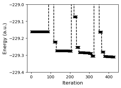
The end result is that we could bring the energy down. Optimizing a basis set is a dangerous game of course, you potentially lose out on a lot of error cancellation and other properties might be negatively affected. How about the band gap?
tn = OptTarget(mol)
tcat = OptTarget(cat)
print("Initial Basis:", h_to_eV*(tn(start_coeff) - tcat(start_coeff)), "eV")
Initial Basis: -8.095511667441343 eV
tn = OptTarget(mol)
tcat = OptTarget(cat)
print("Optimized Basis:", h_to_eV*(tn(opt.x) - tcat(opt.x)), "eV")
Optimized Basis: -8.859976551095974 eV
Not bad, in this case our new basis was able to improve things slightly. There is more to the subject of basis set optimization, such as trying to keep the overlap matrix well conditioned or generation of the gradient, but that will have to be a subject of a future blog post.