Searching for a Reliable Density Functional for Molecule–Environment Interactions, Found B97M-V/def2-mTZVP
I am happy to (belatedly) announce a new publication which I worked on along side Bun Chan and Takahito Nakajima available in the Journal of Physical Chemistry A. In this study, we looked at various low cost density functional protocols for computing the interaction of some small molecules and their surrounding environments. For example, a drug molecule in the pocket of an enzyme.
What do I mean by the word "Protocol"? Well, in the textbook version of Quantum Chemistry calculations, what you would do is pick a method and basis set that are accurate enough for your system, run the calculation, and be done with it. But this might not be practical for your computational resources. So what do you do?
Well, chemists like to cheat. A lot. Let's look at some examples.
Basis Set Extrapolation
The textbook version of cheating might be extrapolating a value to the complete basis set limit.
from pyscf import gto
mstr = """O 0 0 0.1173
          H 0 0.7572 -0.4692
          H 0 -0.7572 -0.4692"""
mol = gto.Mole(atom=mstr)
mol.verbose = 0
Compute the energy with progressively bigger basis sets.
from pyscf import scf
import pickle

energies = {"cc-pVDZ": 0, "cc-pVTZ": 0, "cc-pVQZ": 0, "cc-pV5Z": 0}
try:  # Use Pickle to cache our results.
    with open("energies.pickle", "rb") as ifile:
        energies = pickle.load(ifile)
except:
    for b in energies:
        mol.basis = b
        mol.build()
        mf = scf.RHF(mol)
        energies[b] = mf.kernel()
    with open("energies.pickle", "wb") as ofile:
        pickle.dump(energies, ofile)
And fit the energy to the cardinality of the basis set (in this case, with brute force).
from scipy.optimize import curve_fit
from numpy import exp
fit = lambda x, a, b, c: c + a*exp(-b*x)
coef, _ = curve_fit(fit, [2, 3, 4, 5], [x for x in energies.values()])
Other extrapolation techniques only require two different calculations since they've precomputed some of the constants. I took one example from the website of Dr. Hendrick Zipse. Note that the choice of constants should depend on the method, basis, etc., so I'm really cheating here.
from numpy import sqrt
cbs2 = energies["cc-pVTZ"]*exp(-5.4 * sqrt(3)) - energies["cc-pVQZ"]*exp(-5.4 * sqrt(2))
cbs2 /= exp(-5.4 * sqrt(3)) - exp(-5.4 * sqrt(2))
MRChem is a code based on multi-wavelets, which allows us to very easily specify a target accuracy for a given calculation. We can benchmark our extrapolation by comparing to the MRChem energy.
def compute_mrchem(mstr, mname):
    from json import dump, load
    from os import system
    from os.path import exists

    # Handle conversion of units and format
    def convert_coords(mstr):
        out = ""
        for line in mstr.split("\n"):
            split = line.split()
            pos = [float(x.replace(";",""))*1.88973 for x in split[1:]]
            out += " ".join([split[0]] + [str(x) for x in pos])
            out += "\n"
        return out

    # Parameters
    param = {"world_prec": 1.0e-6,  # Target accuracy
             "WaveFunction": {"method": "HF"},
             "Molecule": {"coords": convert_coords(mstr)}}

    # Write the input file
    with open(mname + ".inp", "w") as ofile:
        dump(param, ofile)

    # Run
    if not exists(mname + ".json"):  # Lazy calculation
        system("mrchem --json " + mname)

    # Return the energy
    with open(mname + ".json") as ifile:
        data = load(ifile)
    return data["output"]["properties"]["scf_energy"]["E_tot"]
mr_val = compute_mrchem(mstr, "h2o")
Plot.
from matplotlib import pyplot as plt
from numpy import linspace
fig, axs = plt.subplots(1, 1, figsize=(5,3))
axs.plot([energies[x] for x in energies], 'k+',
         markersize=12, label="Computed")

xvals = linspace(0, 3.5, 21)
axs.plot(xvals, [fit(x+2, coef[0], coef[1], coef[2]) for x in xvals],
         'r--', label="Fit")
axs.axhline(coef[2], color="olive", linestyle='-',
            label="CBS="+'{0:.6f}'.format(coef[2]))
axs.axhline(mr_val, color="skyblue", linestyle='--', linewidth=1,
            label="CBS2/3="+'{0:.6f}'.format(cbs2))
axs.axhline(mr_val, color="gray", linestyle=':', linewidth=4,
            label="MRChem"+'{0:.6f}'.format(mr_val))

axs.set_xticks(range(len(list(energies))))
axs.set_xticklabels(energies)
axs.set_ylabel("Energy (a.u.)", fontsize=12)
axs.set_xlabel("Basis", fontsize=12)
_ = axs.legend()
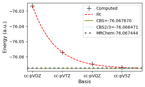
There is a clear trend in the energies as we increase the basis set size. Using the fitting procedure, we can estimate the energy at the complete basis set limit (CBS). When comparing to the MRChem result, either of the CBS extrapolation approaches look quite good.
Molecular Interactions
One case in particular where basis set incompleteness is an issue is for inter-molecular interactions (A + B - AB). In that case, you run into basis set superposition error (BSSE), where the energy of the full system (AB) is artificially lowered because the molecule is represented by the combined basis set of A and B. The counterpoise correction is the classic way to approach this.
ats_a = """O         99.81400      100.83500      101.23200
H         99.32900       99.97700      101.06300
H         99.15200      101.56100      101.41400"""
ats_b = """O        102.36000      101.55100       99.96500
H        102.67500      102.37000      100.44400
H        101.55600      101.18000      100.43000"""
Compute the bare interaction.
interactions = {"def2-SVP": 0, "6-31G*": 0, "cc-pVDZ": 0,
                "cc-pVTZ": 0, "cc-pVQZ": 0, "cc-pV5Z": 0}

try:
    with open("interactions.pickle", "rb") as ifile:
        interactions = pickle.load(ifile)
except:
    for b in interactions:
        mol_a = gto.Mole(atom=ats_a, verbose=0)
        mol_b = gto.Mole(atom=ats_b, verbose=0)
        mol_ab = gto.Mole(atom=ats_a + "\n" + ats_b, verbose=0)

        mol_a.basis = b
        mol_b.basis = b
        mol_ab.basis = b
        mol_a.build()
        mol_b.build()
        mol_ab.build()

        interactions[b] = scf.RHF(mol_a).kernel()
        interactions[b] += scf.RHF(mol_b).kernel()
        interactions[b] -= scf.RHF(mol_ab).kernel()

    with open("interactions.pickle", "wb") as ofile:
        pickle.dump(interactions, ofile)
Compute using the counterpoise correction (ghost atoms).
cpc_interactions = {x: 0 for x in interactions}

try:
    with open("cpc_interactions.pickle", "rb") as ifile:
        cpc_interactions = pickle.load(ifile)
except:
    for b in cpc_interactions:
        mol_a = gto.Mole(atom=ats_a +
                         ats_b.replace("H", "ghost:H").replace("O", "ghost:O"),
                         verbose=0)
        mol_b = gto.Mole(atom=ats_b +
                         ats_a.replace("H", "ghost:H").replace("O", "ghost:O"),
                         verbose=0)
        mol_ab = gto.Mole(atom=ats_a + "\n" + ats_b, verbose=0)

        mol_a.basis = b
        mol_b.basis = b
        mol_ab.basis = b
        mol_a.build()
        mol_b.build()
        mol_ab.build()

        cpc_interactions[b] = scf.RHF(mol_a).kernel()
        cpc_interactions[b] += scf.RHF(mol_b).kernel()
        cpc_interactions[b] -= scf.RHF(mol_ab).kernel()
    with open("cpc_interactions.pickle", "wb") as ofile:
        pickle.dump(cpc_interactions, ofile)
It could be interesting to fit here too.
fit = lambda x, a, b, c: c + a*exp(-b*x)
coef, _ = curve_fit(fit, [2, 3, 4, 5],
                    [x for b, x in interactions.items()
                     if "cc" in b])
Plot a comparison.
fig, axs = plt.subplots(1, 1, figsize=(5,3))
axs.plot([630*interactions[x] for x in interactions], 'k+',
         markersize=12, label="Standard")
axs.plot([630*cpc_interactions[x] for x in interactions], 'rx',
         markersize=12, label="Ghost Atoms")

xvals = linspace(2, 5.5, 21)
axs.plot(xvals, [630*fit(x, coef[0], coef[1], coef[2]) for x in xvals],
         '--', color="skyblue", label="Fit")
axs.axhline(630*coef[2], color="olive", linestyle='-',
            label="CBS="+'{0:.6f}'.format(630*coef[2]))

axs.set_xticks(range(len(list(interactions))))
axs.set_xticklabels(interactions)
axs.set_ylabel("Interaction Energy (kcal/mol)", fontsize=12)
axs.set_xlabel("Basis", fontsize=12)
_ = axs.legend(bbox_to_anchor=(1,1))
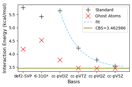
One of the things you can learn from running this notebook is just how expensive calculations get when you use very large basis sets. Fortunately, the counterpoise correction did seem to work quite well here, and would have saved us a lot of time. The downside of the counterpoise correction is an increase in computational cost. This cost may not be worth it, since it might actually remove some favorable error cancellation. In the spirit of cheating, is there something else we can do?
The Geometrical Counterpoise Correction
A very interesting paper came out about a decade ago which proposed a method called "HF-3C". The basic idea was to enable us to compute systems using the simple Hartree-Fock method in a small basis set, by applying 3 empirical corrections: 1) D3 corrections for dispersion; 2) an empirical short range correction; and 3) a correction for basis set incompleteness called the "Geometrical Counterpoise Correction" (GCP). They also used a special version of Huzinga's mini basis set. The paper we published is very much in the spirit of this, as we examined a number of methods which include empirical corrections, as well as modifications to the basis set.
The GCP approach is available in its own separate software package which can be installed via conda (gcp-correction). The GCP program is parameterized for a number of basis sets, and involves a quick pairwise calculation on your set of atoms. Let's try it out with our system.
import subprocess
def get_gcp(fstr, fname, b, nats):
    with open(fname + ".xyz", "w") as ofile:
        ofile.write(str(nats) + "\n\n")
        ofile.write(fstr.replace(";", "") + "\n")

    # Call the program
    ret = subprocess.check_output(["mctc-gcp", fname+".xyz", "-i", "xyz",
                                   "-l", "hf/"+b.replace("*", "s")],
                                  stderr=subprocess.DEVNULL)
    ret = ret.decode('ascii')
    # Extract the energy
    for line in ret.split("\n"):
        if "Egcp" in line:
            return float(line.split()[1])

correction = {}
for b in interactions:
    try:
        gcp_a = get_gcp(ats_a, "mol_a", b, 3)
        gcp_b = get_gcp(ats_b, "mol_b", b, 3)
        gcp_ab = get_gcp(ats_a + "\n" + ats_b, "mol_ab", b, 6)
        correction[b] = gcp_a + gcp_b - gcp_ab
    except subprocess.CalledProcessError:  # Unsupported Basis Sets
        pass
Plot the results.
fig, axs = plt.subplots(1, 1, figsize=(5,3))
axs.plot([630*interactions[x] for x in interactions], 'k+',
         markersize=12, label="Standard")
axs.plot([630*cpc_interactions[x] for x in interactions], 'rx',
         markersize=12, label="Ghost Atoms")
axs.plot([630*(interactions[x] + correction[x]) for x in correction], '1',
         color="olive", markersize=12, label="GCP")

axs.set_xticks(range(len(list(interactions))))
axs.set_xticklabels(interactions)
axs.set_ylabel("Interaction Energy (kcal/mol)", fontsize=12)
axs.set_xlabel("Basis", fontsize=12)
_ = axs.legend(bbox_to_anchor=(1,1))
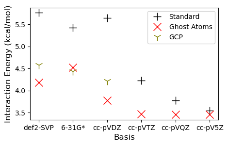
Note the lack of a parameters for the triple-zeta basis and above, this is aimed at cheap calculations. For this example, we find that the GCP has done a good job, giving us essentially triple-$\zeta$ accuracy at a double-$\zeta$ cost, and it runs in an instant. So next time you can't compute a system with the basis/theory you'd like, consider some of the low-cost protocols out there. We had great luck with the r2SCAN-3c and B97M-V/def2-mTZVP combinations.