Sorting drug conformers in enzyme active sites: the XTB way

I have another paper I'd like to share with you that I helped write: Sorting drug conformers in enzyme active sites: the XTB way. The genesis of this paper was that we wanted to try applying quantum chemistry calculations to drug design. We came up with a few interesting targets and got started on our calculations. However, quickly we became concerned about how accurate our methods really were, and how much uncertainty we should expect with respect to experiment. For better of for worse, that got us sidetracked into running more and more benchmarks on systems that looked like our target. These benchmark results are the theme of the paper.

We were very happy to find that the GFN semi-empirical methods available in the XTB Program provided a great balance of accuracy and cost. Of course, these methods have already been evaluated by the people who proposed them and some other groups, but I hope that our results can widen the scope of the evidence, and provide an extra layer of confidence. If you are familiar with the basics of quantum chemistry, I highly recommend you install XTB and try it out on your systems.

Example

Let me provide you a brief illustration of the utility of the GFN methods. Recently I saw a paper published in JCTC that is about the molecules-in-molecules fragment approach. Their focus was on benchmarking fragmentation approaches, but as a side effect they have some useful reference data for us. In their supplementary information there are some benchmarks related to cyclin-dependent kinase 2; the benchmarks include interaction energies computed with three different methods: DLPNO-MP2 cc-pVTZ, DLPNO-MP2 TightPNO def2-TZVP, and DLPNO-CCSD(T) def2-TZVP. Of course, there are various approximations at work here, but let's take their DLPNO-CCSD(T) def2-TZVP value as a benchmark, and see how the other methods compare. I was a little discouraged by the PDF form of the benchmark, but actually ChatGPT was able to extract it for pasting into excel.

from pandas import read_excel
data = read_excel("data.xlsx").to_dict(orient="list")

I've downloaded as well the XYZ files they have provided, so it's a simple matter of looping and computing. We can try out the different GFN methods as we go. I'm going to use our remotemanager library to run this, even though I'm running on my laptop, because it makes it easy to cache the results (so that I can restart my notebook without having to run everything all over again).

def compute(mol, gfn):
    import subprocess
    filename = f"{mol}-{gfn}.out"
    cmd = "ulimit -s hard ; "
    cmd += f'xtb --iterations 5000 {mol}.xyz --{gfn} | tee {filename}'
    cmd += '| grep "TOTAL ENERGY" | ' + "awk '{print $4}'"
    result = subprocess.run(cmd, shell=True, text=True,
                            stderr=subprocess.DEVNULL,
                            stdout=subprocess.PIPE)
    return float(result.stdout.strip())

from remotemanager import Dataset
ds = Dataset(compute, extra_files_send=["CDK2_dataset/*"], verbose=0)
for gfn in ["gfn2", "gfn1"]:
    for mol in data["Molecule ID"]:
        ds.append_run({"mol": mol, "gfn": gfn}, asynchronous=False)
ds.run() ; ds.wait() ; ds.fetch_results()

Put the data back in the table.

data["gfn2"] = []
data["gfn1"] = []
for runner in ds.runners:
    data[runner.args["gfn"]].append(runner.result)

Now transform this data so we get the three point interaction energies.

base = [name for name in data['Molecule ID'] if "Lig" not in name]
ie = {name: {} for name in base}

for n in base:
    ab = data['Molecule ID'].index(n)
    a = data['Molecule ID'].index(n + '_LigOnly')
    b = data['Molecule ID'].index(n + '_NoLig')

    for col in data:
        if col != 'Molecule ID':
            ie[n][col] = data[col][ab] - (data[col][a] + data[col][b])
            ie[n][col] *= 2625.5002  # kJ/mol

Let's create a box plot with the different errors.

from collections import defaultdict
errors = defaultdict(list)
ref = "DLPNO-CCSD(T) def2-TZVP"
for n in base:
    for col in ie[n]:
        if col != ref:
            errors[col].append(ie[n][col] - ie[n][ref])

from matplotlib import pyplot as plt
labels = list(errors.keys())
plt.figure(figsize=(4, 3))
plt.boxplot([errors[method] for method in labels], labels=labels)
plt.ylabel("Error (kJ/mol)")
plt.xticks(rotation=90)

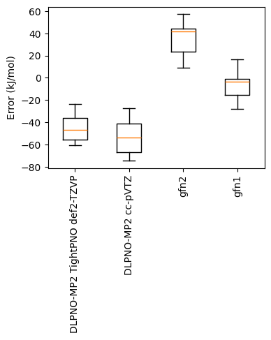
The box plot shows that XTB is performing very well despite being substantially cheaper than the MP2 comparison. GFN1 is so close, one might want to check if it very similar data was included in the original fitting. Relative energies are also an important benchmark though (and remove any constant under / overbinding trend), so let's plot some correlations:

plot_data = {method: {'x': [], 'y': []} for method in ie[base[0]] if method != ref}

for n in base:
    ref_value = ie[n][ref]
    for method in ie[n]:
        if method != ref:
            plot_data[method]['x'].append(ref_value)
            plot_data[method]['y'].append(ie[n][method])

import numpy as np
plt.figure(figsize=(8, 8))

for index, (method, data) in enumerate(plot_data.items(), start=1):
    ax = plt.subplot(2, 2, index)
    x = np.array(data['x'])
    y = np.array(data['y'])

    m, b = np.polyfit(x, y, 1)
    best_fit_line = np.polyval([m, b], x)

    ax.scatter(x, y, color='red')
    ax.plot(x, best_fit_line, color='k')

    ss_res = np.sum((y - best_fit_line) ** 2)
    ss_tot = np.sum((y - np.mean(y)) ** 2)
    r_squared = 1 - (ss_res / ss_tot)

    ax.set_title(f"{method}\n$R^2 = {r_squared:.3f}$")
    ax.set_xlabel(f"{ref}")
    ax.set_ylabel("Computed")

plt.tight_layout()

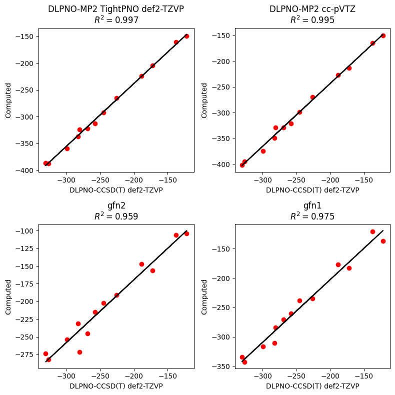
Now we see better the close agreement between MP2 and the reference result. Yet, we shouldn't let this distract us from the remarkable performance of XTB. From looking at the plots, you can definitely imagine deploying XTB over some big datasets to whittle down your focus. Surprisingly, we get better results for the older GFN-1 than GFN-2, which was also true in the paper. For your study, you should definitely try both out to find what works best for you.

Spring 2024

The 2024 cherry blossom season has come and gone here in Japan. Recently, I took a day off to visit Marugame city in Kagawa prefecture. I definitely recommend this city to anyone traveling in the area. This city is famous for Udon... in fact we ate it three times in one day! It also has the beautiful remains of a castle right in the center of the city. I took the below picture from the top, enjoying the view of cherry blossoms and a rather unusally shaped mountain.