Taking Advantage of a Systematic Energy Non-linearity Error in Density Functional Theory for the Calculation of Electronic Energy Levels
I am happy to anounce a new publication which I worked on along side Bun Chan, Takahito Nakajima, and Kimihiko Hirao available in the Journal of Physical Chemistry A. In this paper, we presented a new, low cost scheme for the efficient calculation of electron affinities, ionization potentials, and excitation energies. With this new scheme, even calculations at, say, the BLYP//6-31+G(d) can be sufficient to predict these properties.
To give you a taste of this scheme, I thought I would go through some calculations using PySCF. We will use ionization potentials as the target (refer to the full manuscript for details of other properties). For our system, we will use H2O, which can be setup as such:
from pyscf import gto
sys = gto.Mole()
sys.atom = '''
O 0 0 0.1173 ;
H 0 0.7572 -0.4692 ;
H 0 -0.7572 -0.4692
'''
sys.basis = "6-31+G*"
_ = sys.build()
nocc = int(sys.nelectron / 2)
Hartree-Fock Calculation
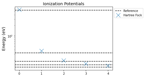
First let's compute the orbital energies with Hartree-Fock. We can compare those energies to the reference ionization potentials found in the Wikipedia article on Koopman's theorem (which will give you more theoertical background): 539.7, 32.2, 18.5, 14.7 and 12.6 eV
reference = [539.7, 32.2, 18.5, 14.7, 12.6]
h_to_ev = 27.2114
from pyscf import scf
mf_hf = scf.RHF(sys)
mf_hf.verbose = 0
mf_hf.kernel()
-76.01625696404005
from matplotlib import pyplot as plt
from matplotlib.ticker import MaxNLocator
fig, axs = plt.subplots(1,1)
label = "Reference"
for v in reference:
    axs.axhline(v, linestyle='--', color='k', label=label)
    label=None
axs.plot([-h_to_ev * x for x in mf_hf.mo_energy[:nocc]],
         marker='x', color="tab:blue", linestyle='None',
         markersize=14, label="Hartree Fock")
axs.set_yscale("log")
axs.set_ylabel("Energy (eV)", fontsize=14)
axs.set_title("Ionization Potentials", fontsize=14)
axs.xaxis.set_major_locator(MaxNLocator(integer=True))
_ = axs.legend(bbox_to_anchor=(1,1))
DFT Calculation
The Hartree-Fock values are actually really good. Now, let's compare that to a DFT calculation like one based on BLYP
from pyscf import dft
mf = dft.RKS(sys)
mf.xc = "BLYP"
mf.verbose = 0
_ = mf.kernel()
fig, axs = plt.subplots(1,1)
label = "Reference"
for v in reference:
    axs.axhline(v, linestyle='--', color='k', label=label)
    label=None
axs.plot([-h_to_ev * x for x in mf_hf.mo_energy[:nocc]],
         marker='x', color="tab:blue", linestyle='None',
         markersize=14, label="Hartree Fock")
axs.plot([-h_to_ev * x for x in mf.mo_energy[:nocc]],
         marker='+', color="tab:orange", linestyle='None',
         markersize=14, label="DFT (BLYP)")
axs.set_yscale("log")
axs.set_ylabel("Energy (eV)", fontsize=14)
axs.set_title("Ionization Potentials", fontsize=14)
axs.xaxis.set_major_locator(MaxNLocator(integer=True))
_ = axs.legend(bbox_to_anchor=(1,1))
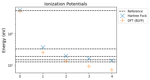
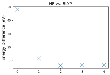
The DFT result is significantly worse than the Hartree-Fock one. Narrowing in, we can look at our accuracy of the first ionization potential
estimate_hf = (h_to_ev * mf_hf.mo_energy[nocc-1])
estimate_dft = (h_to_ev * mf.mo_energy[nocc-1])

print("Type", "Estimate", "Error")
print("Hartree-Fock:", estimate_hf, -reference[-1] - estimate_hf)
print("DFT:", estimate_dft, -reference[-1] - estimate_dft)
Type Estimate Error
Hartree-Fock: -13.863945084275324 1.2639450842753241
DFT: -7.075046911926883 -5.524953088073117
And see that the magnitude of the error is quite substantial. We can also see visually that the error is not just based on a constant shift.
fig, axs = plt.subplots(1,1)
axs.plot([abs(h_to_ev * (x - y)) for x, y in
          zip(mf_hf.mo_energy[:nocc], mf.mo_energy[:nocc])],
         marker='x', color="tab:blue", linestyle='None',
         markersize=14)
axs.set_ylabel("Energy Difference (eV)", fontsize=14)
axs.set_title("HF vs. BLYP", fontsize=14)
axs.xaxis.set_major_locator(MaxNLocator(integer=True))
Cation Calculation
One other way to estimate the first ionization potential is to use $ \Delta $SCF. Here we compute H2O+, so that we might compute the energy difference.
sys_p = sys.copy()
sys_p.charge = 1
sys_p.spin = 1
_ = sys_p.build()
mf_p = dft.UKS(sys_p)
mf_p.xc = "BLYP"
mf_p.verbose = 0
_ = mf_p.kernel()
estimate_dscf = h_to_ev * (mf.e_tot - mf_p.e_tot)
print("Type", "Estimatate", "Error")
print("Hartree-Fock:", estimate_hf, -reference[-1] - estimate_hf)
print("DFT:", estimate_dft, -reference[-1] - estimate_dft)
print("Delta SCF:", estimate_dscf, -reference[-1] - estimate_dscf)
Type Estimatate Error
Hartree-Fock: -13.863945084275324 1.2639450842753241
DFT: -7.075046911926883 -5.524953088073117
Delta SCF: -12.702624320794662 0.10262432079466244
That is the most accurate method yet. Now, from the calculation of H2O+, we can also try to estimate the ionization potential by looking at the LUMO.
estimate_p = h_to_ev * mf_p.mo_energy[1, nocc - 1]
print("Type", "Estimatate", "Error")
print("Hartree-Fock:", estimate_hf, -reference[-1] - estimate_hf)
print("DFT:", estimate_dft, -reference[-1] - estimate_dft)
print("Delta SCF:", estimate_dscf, -reference[-1] - estimate_dscf)
print("DFT (+):", estimate_p, -reference[-1] - estimate_p)
Type Estimatate Error
Hartree-Fock: -13.863945084275324 1.2639450842753241
DFT: -7.075046911926883 -5.524953088073117
Delta SCF: -12.702624320794662 0.10262432079466244
DFT (+): -18.43253533561162 5.832535335611622
The calculation of H2O+ gives a similar error to our DFT calculation of H2O. But interestingly, the error has the opposite sign. This suggests that we can combine the estimates to get an accurate result.
combined = estimate_dft + 0.5 * (estimate_p - estimate_dft)
print("Type", "Estimatate", "Error")
print("Hartree-Fock:", estimate_hf, -reference[-1] - estimate_hf)
print("DFT:", estimate_dft, -reference[-1] - estimate_dft)
print("Delta SCF:", estimate_dscf, -reference[-1] - estimate_dscf)
print("DFT (+):", estimate_p, -reference[-1] - estimate_p)
print("DFT (Combined):", combined, -reference[-1] - combined)
Type Estimatate Error
Hartree-Fock: -13.863945084275324 1.2639450842753241
DFT: -7.075046911926883 -5.524953088073117
Delta SCF: -12.702624320794662 0.10262432079466244
DFT (+): -18.43253533561162 5.832535335611622
DFT (Combined): -12.753791123769252 0.15379112376925264
Correction Approach
In our approach, this averaging leads to a correction term, which can then be applied to other orbitals. Let's see how this approach fares.
correction = combined - estimate_dft
corrected = [h_to_ev * x + correction for x in mf.mo_energy]
fig, axs = plt.subplots(1,1)
label = "Reference"
for v in reference:
    axs.axhline(v, linestyle='--', color='k', label=label)
    label=None
axs.plot([-h_to_ev * x for x in mf_hf.mo_energy[:nocc]],
         marker='x', color="tab:blue", linestyle='None',
         markersize=14, label="Hartree Fock")
axs.plot([-h_to_ev * x for x in mf.mo_energy[:nocc]],
         marker='+', color="tab:orange", linestyle='None',
         markersize=14, label="DFT (BLYP)")
axs.plot([-1 * x for x in corrected[:nocc]],
         marker='*', color="tab:green", linestyle='None',
         markersize=14, label="Corrected")
axs.set_yscale("log")
axs.set_ylabel("Energy (eV)", fontsize=14)
axs.set_title("Ionization Potentials", fontsize=14)
axs.xaxis.set_major_locator(MaxNLocator(integer=True))
_ = axs.legend(bbox_to_anchor=(1,1))
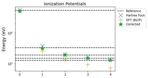
This simple correction has improved our estimate of the ionization energy for all orbitals. Let's look closer at the actual error.
fig, axs = plt.subplots(1,1)
axs.plot([abs(-1 * x - y) for x, y in zip(mf_hf.mo_energy[:nocc], reference)],
         marker='x', color="tab:blue", linestyle='None',
         markersize=14, label="Hartree-Fock")
axs.plot([abs(-1 * x - y) for x, y in zip(corrected[:nocc], reference)],
         marker='*', color="tab:green", linestyle='None',
         markersize=14, label="Corrected")
axs.plot(nocc - 1, -reference[-1] - estimate_dscf,
         marker='o', color="tab:red", linestyle='None',
         label="Delta SCF")
axs.set_ylabel("(ABS) Error (eV)", fontsize=14)
axs.set_title("Ionization Potential Errors", fontsize=14)
axs.set_yscale("log")
axs.xaxis.set_major_locator(MaxNLocator(integer=True))
_ = axs.legend(bbox_to_anchor=(1,1))
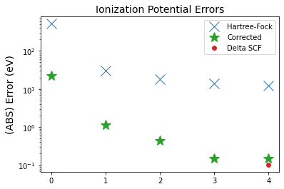
While the error is good, it isn't balanced, with the core orbital having a very big error. So, in this paper we further propose a scaling factor for the correction based on the exchange energy of a given orbital. This scaling factor can be computed using some of the machinery in PySCF.
ni = dft.numint.NumInt()
grids = dft.gen_grid.Grids(sys)
grids.level = 4
_ = grids.build()
from numpy import outer
scaling = []
for i in range(nocc):
    mo = mf.mo_coeff[:, i]
    dm = outer(mo, mo)
    _, exc, _ = ni.nr_rks(sys, grids, 'lda,', dm)
    scaling.append(exc)
Then we apply the new correction which scales by this factor.
new_corrected = [h_to_ev * x + scaling[i]/scaling[-1] * correction
                 for i, x in enumerate(mf.mo_energy[:nocc])]
fig, axs = plt.subplots(1,1)
axs.plot([abs(-1 * x - y) for x, y in zip(mf_hf.mo_energy[:nocc], reference)],
         marker='x', color="tab:blue", linestyle='None',
         markersize=14, label="Hartree-Fock")
axs.plot([abs(-1 * x - y) for x, y in zip(corrected[:nocc], reference)],
         marker='*', color="tab:green", linestyle='None',
         markersize=14, label="Corrected")
axs.plot([abs(-1 * x - y) for x, y in zip(new_corrected[:nocc], reference)],
         marker='P', color="tab:purple", linestyle='None',
         markersize=14, label="New Corrected")
axs.plot(nocc - 1, -reference[-1] - estimate_dscf,
         'yo', label="Delta SCF")
axs.set_ylabel("(ABS) Error (eV)", fontsize=14)
axs.xaxis.set_major_locator(MaxNLocator(integer=True))
axs.set_yscale("log")
_ = axs.legend(bbox_to_anchor=(1,1))
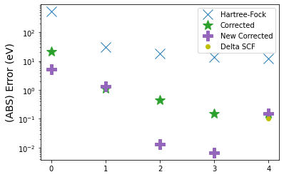
The scaled version does seem to improve on a number of orbitals! In the paper, you will find more validation, and a theoretical description of what's actually going on. But I hope that this re-implementation of our analysis using the very friendly API of PySCF gives you a more hands on feel of our results.
Chan, Bun, William Dawson, Takahito Nakajima, and Kimihiko Hirao. "Taking Advantage of a Systematic Energy Non-linearity Error in Density Functional Theory for the Calculation of Electronic Energy Levels." The Journal of Physical Chemistry A (2021).