Towards Routine Orbital-Free Large-Scale Quantum-Mechanical Modelling of Materials
Last week, I got to participate in a workshop Towards Routine Orbital-free Large-Scale Quantum-Mechanical Modelling of Materials held in Hangzhou, China. Orbital-Free Density Functional Theory (OF-DFT) is an attractive alternative to the far more popular Kohn-Sham Density Functional Theory:
$$\begin{equation} E[\rho] = T_s[\rho] + E_H[\rho] + E_{ext}[\rho] + \int v_{ext}\rho(r)dr \end{equation}$$
Here $T_s$ is the kinetic energy density functional - deriving approximations to this term is the hardest part of OF-DFT development. At the workshop, one of the speakers presented their own OF-DFT package: DFTpy. Experimenting with this software could be a good way to spend this blog post.
But first, photos of China.


Calculation Setup
DFTpy already has an ASE calculator, so we can use that as a base for comparison to our Kohn-Sham BigDFT code.
The calculations (especially with BigDFT) are non-trivial so let's setup remotemanager to do this on my local cluster.
from remotemanager import RemoteFunction, SanzuFunction
from spring import Spring
url = Spring()
url.mpi = 4
url.omp = 9
url.queue = "winter2"
url.conda = "bdft"
url.path_to_bigdft = "/home/dawson/binaries/bdft/"
First, make a system of bulk magnesium.
A = 3.2091 # taken from Wikipedia
C = 5.2103
@RemoteFunction
def make_ase(a=A, c=C):
    from ase.build import bulk
    asys = bulk("Mg", crystalstructure="hcp", orthorhombic=True,
                a=a, c=c)
    return asys
Visualize this using PyBigDFT.
@RemoteFunction
def make_system(a=A, c=C):
    from BigDFT.Systems import System
    from BigDFT.UnitCells import UnitCell
    from BigDFT.Interop.ASEInterop import ase_to_bigdft, \
         ase_cell_to_bigdft

    # Build with ASE
    asys = make_ase(a, c)

    # Convert to BigDFT
    sys = System()
    sys["FRA:0"] = ase_to_bigdft(asys)
    sys.cell = ase_cell_to_bigdft(asys.cell)

    return sys
sys = make_system()
_ = sys.display()
3Dmol.js failed to load for some reason. Please check your browser console for error messages.
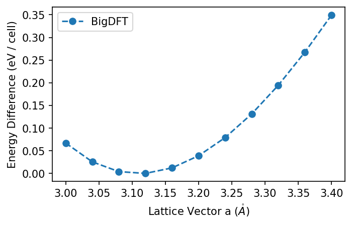
Using BigDFT, we can compute a potential energy curve by varying the lattice vectors. Let's try varying a.
from numpy import linspace
avals = linspace(3, 3.4, 11)
@SanzuFunction(url=url, name="bigdft", verbose=False)
def calculate(a, pts, name):
    from BigDFT.Inputfiles import Inputfile
    from BigDFT.Calculators import SystemCalculator

    calc = SystemCalculator(skip=True)
    sys = make_system(a=a)

    inp = Inputfile()
    inp.set_xc("LDA")
    inp.set_hgrid(0.35)
    inp.set_psp_krack(functional="LDA")
    inp["kpt"] = {"method": "mpgrid", "ngkpt": pts}
    inp["import"] = "mixing" # because it's a metal

    log = calc.run(sys=sys, input=inp, name=name, run_dir="scr")
    return log.energy
results = {}
for i, a in enumerate(avals):
    results[a] = calculate(a, [6, 4, 4], f"bigdft-{i}")
Plot the change in energy per unit cell.
def plot_all(data):
    from matplotlib import pyplot as plt
    fig, axs = plt.subplots(1, 1, dpi=150, figsize=(5, 3))
    for k, v in data.items():
        minv = min(v.values())
        axs.plot(avals, [27.2114 * (v[x] - minv) for x in avals],
                 'o--', label=k)
    axs.set_ylabel("Energy Difference (eV / cell)")
    axs.set_xlabel("Lattice Vector a ($\mathring{A}$)")
    axs.legend()
plot_all({"BigDFT": results})
Orbital-Free Comparison
Ok now let's try to do the same thing with OF-DFT and DFTpy. To do this, we're going to need a local pseudopotential for use with OF-DFT. We can use the BLPS library of pseudopotentials for this test.
from os import system
pp = "https://raw.githubusercontent.com/PrincetonUniversity/BLPSLibrary/master/LDA/reci/mg.lda.recpot"
_ = system(f"mkdir -p pp; cd pp; wget {pp} 2>/dev/null")
And prepare to run DFTpy.
# mpi parallel version is also available
url.omp = 1
url.mpi = 1
@SanzuFunction(url=url, name="of-dft", verbose=False, extra_files_send="pp")
def calculate_of(a, pts, name, kedf):
    from ase.io import write
    from futile.Utils import ensure_dir
    from shutil import copyfile
    from os import system

    # no built in toml writer...
    def dump(inp, ofile):
        for h, ent in inp.items():
            ofile.write(f"[{h}]\n")
            for k, v in ent.items():
                ofile.write(f"{k}={v}\n")

    # create the system
    asys = make_ase(a=a)
    asys = asys * pts  # build the supercell instead of k-points

    # write the files to the scratch directory
    ensure_dir("scr-of")
    write(f"scr-of/{name}.vasp", asys)
    copyfile("pp/mg.lda.recpot", "scr-of/mg.lda.recpot")

    # create the input file
    inp = {}
    inp["PP"] = {"Mg": "mg.lda.recpot"}
    inp["CELL"] = {"cellfile": f"{name}.vasp"}
    inp["GRID"] = {"spacing": 0.3}
    inp["EXC"] = {"xc": "LDA"}
    inp["KEDF"] = {"kedf": kedf}
    with open(f"scr-of/{name}.ini", "w") as ofile:
        dump(inp, ofile)

    # run the calculation
    system(f"cd scr-of ; python -m dftpy {name}.ini > {name}.log")

    # grab the energy
    with open(f"scr-of/{name}.log") as ifile:
        for line in ifile:
            if "total energy (a.u.)" in line:
                # divide to get the per unit cell contribution
                return float(line.split()[-1]) / (pts[0] * pts[1] * pts[2])
DFTpy can also be used purely from python but this use of it as an executable matches our BigDFT workflow well. Now let's run the calculations and compare.
results_of = {"TFvW": {}}
for i, a in enumerate(avals):
    results_of["TFvW"][a] = calculate_of(a, [6, 4, 4], f"of-{i}", "TFvW")
plot_all({"BigDFT": results,
          "TFvW": results_of["TFvW"]})
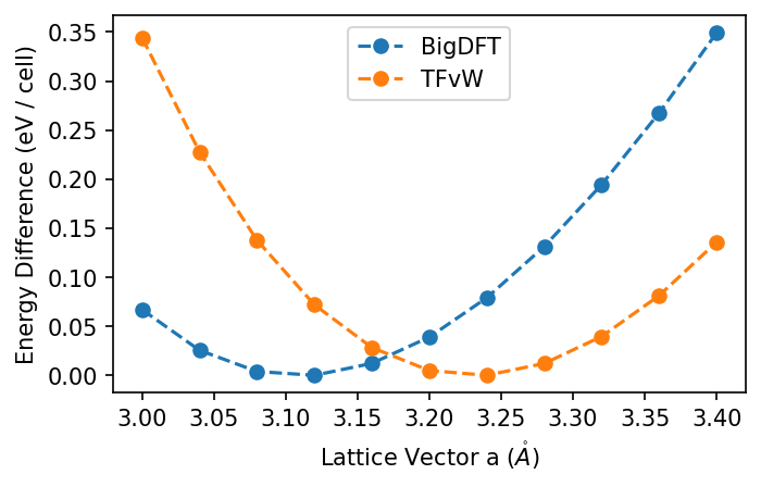
We might wonder if a different kinetic energy functional would match closer to BigDFT. In particular, we can try a non-local functional.
results_of["MGPA"] = {}
for i, a in enumerate(avals):
    results_of["MGPA"][a] = calculate_of(a, [6, 4, 4], f"of-{i}", "MGPA")
plot_all({"BigDFT": results,
          "TFvW": results_of["TFvW"],
          "MGPA": results_of["MGPA"]})
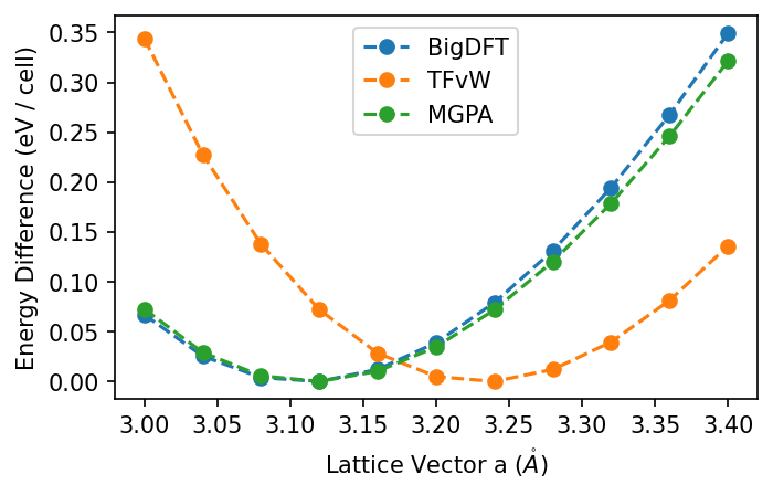
This functional indeed matches closer to our BigDFT results - though who is ultimately correct is a different matter. OF-DFT has the benefit of being much cheaper to calculate (it is linear scaling with a low prefactor). With this in mind, it could be interesting to use it to study size dependent effects of systems, with BigDFT's linear scaling mode as a means of checking the result.